Page 529 - Fiber Optic Communications Fund

510 Fiber Optic Communications

Solution:
For a 10-GSym/s system, the symbol period is 100 ps. Since there are two samples per symbol, T samp = 50 ps.
Using Eq. (11.64), we find
( −27 3 )
× 22 × 10 × 800 × 10
K = ceil = 23. (11.65)
)
(50 × 10 −12 2
Therefore, the number of taps 2K + 1 = 47.

11.6.1 Adaptive Equalizers
The fiber dispersion could fluctuate due to environmental conditions. However, these fluctuations occur at
a rate that is much slower than the transmission data rate and, therefore, the tap weights of the FIR filter
shown in Fig. 11.13 can be adjusted adaptively. There exist a number of techniques to realize the tunable
dispersion-compensating filters [18–20]. In this section, we focus on two types of adaptive equalizer: least
mean squares (LMS) and constant modulus algorithm (CMA) equalizers.
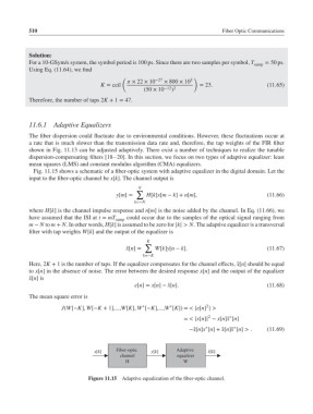
Fig. 11.15 shows a schematic of a fiber-optic system with adaptive equalizer in the digital domain. Let the
input to the fiber-optic channel be x[k]. The channel output is
N
∑
y[m]= H[k]x[m − k]+ n[m], (11.66)
k=−N
where H[k] is the channel impulse response and n[m] is the noise added by the channel. In Eq. (11.66), we
have assumed that the ISI at t = mT could occur due to the samples of the optical signal ranging from
samp
m − N to m + N. In other words, H[k] is assumed to be zero for |k| > N. The adaptive equalizer is a transversal
filter with tap weights W[k] and the output of the equalizer is
K
∑
̂ x[n]= W[k]y[n − k]. (11.67)
k=−K
Here, 2K + 1 is the number of taps. If the equalizer compensates for the channel effects, ̂x[n] should be equal
to x[n] in the absence of noise. The error between the desired response x[n] and the output of the equalizer
̂ x[n] is
e[n]= x[n]− ̂x[n]. (11.68)
The mean square error is
2
∗
∗
J(W[−K], W[−K + 1],...,W[K], W [−K],...,W [K]) = < |e[n] | >
2
∗
= < |x[n]| − x[n]̂x [n]
∗ ∗
−̂x[n]x [n]+ ̂x[n]̂x [n] >. (11.69)
x[k] Fiber-optic y[k] Adaptive ˆ x[k]
channel equalizer
H W

Figure 11.15 Adaptive equalization of the fiber-optic channel.