Page 528 - Fiber Optic Communications Fund

Digital Signal Processing 509

0.15 0.1
0.1 0.05
Quad. comp. (a.u.) *0.05 0 Quad. comp. (a.u.) 0
0.05

*0.1
*0.15 *0.05

*0.2 *0.1
*0.2 *0.1 0 0.1 0.2 *0.1 *0.05 0 0.05 0.1
In−phase (a.u.) In−phase (a.u.)
(a)
(b)
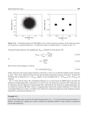
Figure 11.14 Constellation diagrams for NRZ-QPSK system: (a) before dispersion equalizer, (b) after dispersion equal-
izer. Parameters: accumulated dispersion = 13, 600 ps/nm, number of samples/symbol = 2, number of taps = 47.

Using the Nyquist theorem, the sampling rate, R samp , should be at least equal to 2B,

1 KT samp
R = ≥ (11.62)
samp
T | |L
samp 2
or
| |L
2
K ≥ . (11.63)
T 2
samp
Since K has to be an integer, we choose
2
K = ceil(| |L∕T samp ), (11.64)
2
where ceil() gives the nearest integer toward ∞. From Eq. (11.64), we see that the number of taps increases
as | |L. This can be understood from the fact that the pulse broadening increases with | |L. To undo the
2
2
distortion due to dispersion at t = kT samp , samples of y(t) extending from (k − K)T samp to (k + K)T samp are
required.
Fig. 11.14(a) and (b) shows the constellation diagrams of a system based on QPSK before and after the
dispersion-compensating filter, respectively. As can be seen, the distortions caused by fiber dispersion can
be mitigated using the dispersion-compensating filter. Alternatively, the dispersion-compensating filter can
be realized by using an IIR filter, which is computationally efficient but requires buffering [17]. When the
accumulated dispersion is large, it would be more efficient to compensate dispersion in the frequency domain
using FFTs, as discussed in Section 11.8.

Example 11.1
2
A 10-GSym/s fiber-optic system has the following parameters: =−22 ps ∕km and transmission distance =
2
800 km. Assuming two samples per symbol, calculate the minimum number of taps needed to compensate
for the fiber dispersion.