Page 526 - Fiber Optic Communications Fund

Digital Signal Processing 507

̃
where x(t) is the input field envelope of the fiber and H(f) is the fiber transfer function. The dispersion-
compensating filter (DCF) should have the transfer function
1
̃
W(f)= , (11.45)
̃
H(f)
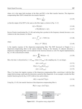
so that the output of the DCF is the same as the fiber input, as shown in Fig. 11.12:
̃
̂ x(f)= W(f)̃y(f) (11.46)
̃
̃
= W(f)H(f)̃x(f)= ̃x(f). (11.47)
Inverse Fourier transforming Eq. (11.46) and noting that a product in the frequency domain becomes a con-
volution in the time domain, we obtain
∞
′
′
x(t)= y(t − t )W(t ) dt, (11.48)
∫
−∞
where
W(t)=  −1 ̃ (11.49)
[W(f)]
is the impulse response of the dispersion-compensating filter. The DCF discussed in Chapter 2 is a
dispersion-compensating filter in the optical domain. Owing to the linearity of coherent detection, a
dispersion-compensating filter can be realized in the electrical domain as well. For digital implementation,
Eq. (11.48) is discretized to obtain
∞
∑
x[n]= W[k]y[n − k]. (11.50)
k=−∞
Here, the time t is discretized as t = kT , where 1∕T is the sampling rate, k is an integer,
samp samp
x[n]= x(nT ), (11.51)
samp
W[n]= T samp W(nT samp ), (11.52)

y[n]= y(nT ). (11.53)
samp
Thus, if we know the impulse response of the dispersion-compensating filter, convolving it with the fiber
output field envelope could undo the distortions caused by fiber dispersion. As an example, consider the fiber
transfer function given by Eq. (2.107) (with no loss and no delay),

2 2
H(f)= exp (i2 f L). (11.54)
2
Using Eq. (11.45), the transfer function of the dispersion-compensating filter is
̃
2 2
W(f)= exp (−i2 f L). (11.55)
2

ˆ
˜
x( f ) Fiber y( f ) Disp. x( f ) = x ( f )
˜
˜
compensation
˜
˜
H( f ) filter W( f )
Figure 11.12 CD equalizer using a digital DCF.