Page 522 - Fiber Optic Communications Fund

Digital Signal Processing 503

0.06 0.06
0.04 0.04
Quad. comp. (a.u.) *0.02 0 Quad. comp. (a.u.) *0.02 0
0.02
0.02

*0.04
*0.06 *0.04
*0.06
*0.1 *0.05 0 0.05 0.1 *0.1 *0.05 0 0.05 0.1
In-phase (a.u.) In-phase (a.u.)
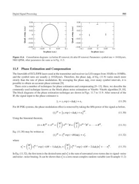
Figure 11.6 Constellation diagrams: (a) before IF removal, (b) after IF removal. Parameters: symbol rate = 10 GSym/s,
NRZ-QPSK, other parameters the same as in Fig. 11.5.

11.5 Phase Estimation and Compensation
The linewidth of ECL/DFB lasers used at the transmitter and receiver (as LO) ranges from 10 kHz to 10 MHz,
and the symbol rates are usually ≥ 10 GSym/s. Therefore, the phase Δ of Eq. (11.9) varies much more
k
slowly than the rate of phase modulation. By averaging the phase Δ over many symbol intervals, it is
k
possible to obtain an accurate phase estimate [9].
There exist a number of techniques for phase estimation and compensating [9–13]. Here, we describe the
commonly used technique known as the block phase noise estimation or Viterbi–Viterbi algorithm [9, 10].
The block diagrams of the phase estimation technique are shown in Figs. 11.7 to 11.9. After removal of the
IF, the signal input to the phase estimator is

̃ y = x exp (−iΔ )+ n . (11.29)
l
l
l
l
For M-PSK systems, the phase modulation effect is removed by taking the Mth power of the signal as before,
[ ] M
M
( ̃y ) = x exp (−iΔ )+ n l . (11.30)
l
l
l
Using the binomial theorem,
( ) ( )
M M
M M M−1 M−2 2 M
(A + B) = A + A B + A B +···+ B , (11.31)
1 2
Eq. (11.30) may be written as
M
M
′
( ̃y ) = x exp (−iMΔ )+ n , (11.32)
l
l
l
l
where
( ) ( )
M M−1 M M−2 2 M
′
n = x exp [−i(M − 1)Δ ]n + x exp [−i(M − 2)Δ ]n +··· n . (11.33)
l 1 l l l 2 l l l l
′
In Eq. (11.32), the first term is the desired term and n is the sum of unwanted cross-terms due to signal–noise
l
′
and noise–noise beating. It can be shown that n is a zero-mean complex random variable (see Example 11.2)
l