Page 517 - Fiber Optic Communications Fund

498 Fiber Optic Communications

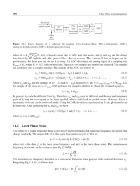
Received
y I y I,l
optical signal 90° PDs ADC
Hybrid and y Q y Q,l DSP
front end ADC
LO

Figure 11.1 Block diagram of a coherent IQ receiver. LO = local oscillator, PDs = photodiodes, ADC =
analog-to-digital converter, DSP = digital signal processing.

√
where K = R P P ∕2, n(t) represents noise due to ASE and shot noise, and and are the delays
r LO I Q
∘
introduced by 90 hybrids and other parts of the coherent receiver. The constant K has no impact on the
performance. So, from now on, we set it to unity. An ADC discretizes the analog signal at a sampling rate
R samp ≥ B , where B = 1∕T is the symbol rate. Typically, two samples per symbol are required. The samples
s
s
s
are combined into a complex number. The outputs of the ADC are written as
y = Re{s exp [−i(2f (t − )+Δ )] + n }, (11.6)
I,l I,l IF l I,l l l
y Q,l = Im{s Q,l exp [−i(2f (t − )+Δ )] + n }, l = 1, 2, … , (11.7)
Q,l
IF l
l
l
where s and s are the samples of s(t − ) and s(t − ), respectively, at t = lT , T = 1∕R . n is
I,l Q,l I Q samp samp samp l
the sample of the noise at t = lT . DSP performs the complex addition to obtain the received signal as
samp
y = y + iy . (11.8)
l I,l Q,l
In general, could be different from . Therefore, s and s may be different, and the real and imaginary
I Q I,l Q,l
parts of ̃y may not correspond to the same symbol, which could lead to symbol errors. However, this is a
l
systematic error and can be corrected easily. Using the DSP, the delays experienced by I- and Q-channels can
be removed. After correcting for and ,wehave
I Q
y = x exp [−i(2f t +Δ )] + n , l = 1, 2, … , (11.9)
l l IF l l l
where x = s ≡ s(lT samp ).
l
l
11.3 Laser Phase Noise
The output of a single-frequency laser is not strictly monochromatic but rather has frequency deviations that
change randomly. The output field of a fiber-optic transmitter may be written as
q (t)= A s(t) exp {−i[2f t − (t)]}, (11.10)
T T c
where s(t) is the data, f is the laser mean frequency, and (t) is the laser phase noise. The instantaneous
c
frequency deviation can be written as (see Eq. (2.165))
1 d
f =− . (11.11)
i
2 dt
The instantaneous frequency deviation is a zero-mean Gaussian noise process with standard deviation .
f
Integrating Eq. (11.11), it follows that
t
(t)= (t )− 2 ∫ f ()d (11.12)
0
i
t 0