Page 76 - Fiber Optic Communications Fund

Optical Fiber Transmission 57

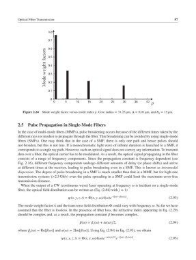
Figure 2.24 Mode weight factor versus mode index p. Core radius = 31.25 μm, Δ= 0.01 μm, and R = 15 μm.
0

2.5 Pulse Propagation in Single-Mode Fibers

In the case of multi-mode fibers (MMFs), pulse broadening occurs because of the different times taken by the
different rays (or modes) to propagate through the fiber. This broadening can be avoided by using single-mode
fibers (SMFs). One may think that in the case of a SMF, there is only one path and hence pulses should
not broaden, but this is not true. If a monochromatic light wave of infinite duration is launched to a SMF, it
corresponds to a single ray path. However, such an optical signal does not convey any information. To transmit
data over a fiber, the optical carrier has to be modulated. As a result, the optical signal propagating in the fiber
consists of a range of frequency components. Since the propagation constant is frequency dependent (see
Fig. 2.16), different frequency components undergo different amounts of delay (or phase shifts) and arrive
at different times at the receiver, leading to pulse broadening even in a SMF. This is known as intramodal
dispersion. The degree of pulse broadening in a SMF is much smaller than that in a MMF, but for high-rate
transmission systems (>2.5 Gb/s) even the pulse spreading in a SMF could limit the maximum error-free
transmission distance.
When the output of a CW (continuous wave) laser operating at frequency is incident on a single-mode
fiber, the optical field distribution can be written as (Eq. (2.84) with j = 1)

(x, y, z, t)=Φ(x, y,)A()e −i[t−()z] . (2.93)
The mode weight factor A and the transverse field distribution Φ could vary with frequency . So far we have
assumed that the fiber is lossless. In the presence of fiber loss, the refractive index appearing in Eq. (2.29)
should be complex and, as a result, the propagation constant becomes complex,

()= ()+ i()∕2, (2.94)
r
where ()= Re[()] and ()= 2Im[()]. Using Eq. (2.94) in Eq. (2.93), we obtain
r
e
(x, y, z, t)=Φ(x, y,)A()e −()z∕2 −i[t− r ()z] . (2.95)