Page 79 - Fiber Optic Communications Fund

60 Fiber Optic Communications

S i (t) S o (t)
H (Ω, L)
f
~ ~ ~
S (Ω) S (Ω) = S i (Ω)H f (Ω, L)
i
o
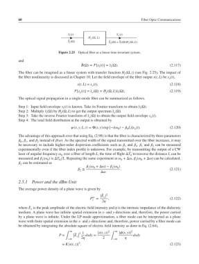
Figure 2.25 Optical fiber as a linear time-invariant system.
and
̃
B(Ω) = [s (t)] = ̃s (Ω). (2.117)
i i
The fiber can be imagined as a linear system with transfer function H (Ω, z) (see Fig. 2.25), The impact of
f
the fiber nonlinearity is discussed in Chapter 10. Let the field envelope of the fiber output s(t, L) be s (t),
o
s(t, L)= s (t), (2.118)
o
[s (t)] = ̃s (Ω) = H (Ω, L)̃s (Ω). (2.119)
o o f i
The optical signal propagation in a single-mode fiber can be summarized as follows.

Step 1: Input field envelope s (t) is known. Take its Fourier transform to obtain ̃s (Ω).
i
i
Step 2: Multiply ̃s (Ω) by H (Ω, L) to get the output spectrum ̃s (Ω).
i f o
Step 3: Take the inverse Fourier transform of ̃s (Ω) to obtain the output field envelope s (t).
o o
Step 4: The total field distribution at the output is obtained by
(x, y, L, t)=Φ(x, y) exp [−i( t − L)]s (t). (2.120)
0 0 o
The advantage of this approach over that using Eq. (2.98) is that the fiber is characterized by three parameters
, , and instead of (). As the spectral width of the signal transmitted over the fiber increases, it may
0 1 2
be necessary to include higher-order dispersion coefficients such as and . and can be measured
3 4 1 2
experimentally even if the fiber index profile is unknown. For example, by transmitting the output of a CW
laser of angular frequency over a fiber of length L, the time of flight ΔT to traverse the distance L can be
0 0
measured and ( ) is ΔT ∕L. Repeating the same experiment at +Δ, ( +Δ) can be calculated.
0
0
1
0
0
1
can be estimated as
2
( +Δ)− ( )
1
0
1
0
≅ . (2.121)
2
Δ
2.5.1 Power and the dBm Unit
The average power density of a plane wave is given by
̃ x 2
|E |
av
P = , (2.122)
z
2
̃
where E is the peak amplitude of the electric field intensity and is the intrinsic impedance of the dielectric
x
medium. A plane wave has infinite spatial extension in x- and y-directions and, therefore, the power carried
by a plane wave is infinite. Under the LP-mode approximation, a fiber mode can be interpreted as a plane
wave with finite spatial extension in the x- and y-directions and, therefore, power carried by a fiber mode can
be obtained by integrating the absolute square of electric field intensity as done in Eq. (2.64),
∞ 2 1 2 ∞ 2
E
P = | ̃ | dxdy = |s(t, z)| |(x, y)| dxdy
∫ | x| ∫
−∞ 2 2 −∞
2
= K|s(t, z)| . (2.123)