Page 84 - Fiber Optic Communications Fund

Optical Fiber Transmission 65

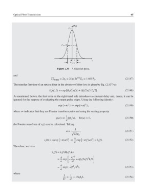
Figure 2.31 A Gaussian pulse.

and
T in = 2t = 2(ln 2) 1∕2 T ≃ 1.665T . (2.147)
FWHM h 0 0
The transfer function of an optical fiber in the absence of fiber loss is given by Eq. (2.107) as

2
H (f, L)= exp [i (2f)L + i (2f) L∕2]. (2.148)
f 1 2
As mentioned before, the first term on the right-hand side introduces a constant delay and, hence, it can be
ignored for the purpose of evaluating the output pulse shape. Using the following identity:
( 2 ) ( 2 )
exp −t ⇌ exp −f , (2.149)
where ⇌ indicates that they are Fourier transform pairs and using the scaling property

1
g(at) ⇌ ̃ g(f∕a), Re(a) > 0, (2.150)
a
the Fourier transform of s (t) can be calculated. Taking
i
1
a = √ , (2.151)
2T
0
[ 2 ] A [ 2 ]
s (t)= A exp −(at) ⇌ exp −(f∕a) = ̃s (f). (2.152)
i i
a
Therefore, we have
̃ s (f)= ̃s (f)H (f, L)
f
i
o
[ 2 ]
A f 2
= exp − + i (2f) L∕2
2
a a 2
A 2 2
= exp (−f ∕b ), (2.153)
a
where
1 1
= − i2 L. (2.154)
2
b 2 a 2