Page 82 - Fiber Optic Communications Fund

Optical Fiber Transmission 63

Figure 2.27 In free space, the pulse shape does not change.

Step 3: The delay in time domain corresponds to a constant phase shift in frequency domain,

g(t − T ) ⇌ ̃g(f) exp (i2fT ). (2.137)
0
0
Using Eqs. (2.134) and (2.136), the output field envelope may be written as
( )
t − L
1
s (t)= s (t − L)= rect . (2.138)
i
o
1
T 0
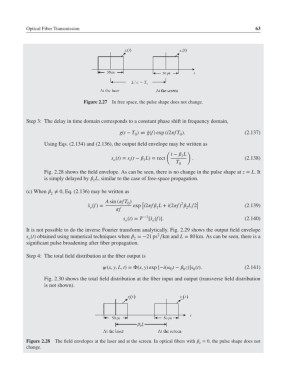
Fig. 2.28 shows the field envelope. As can be seen, there is no change in the pulse shape at z = L.It
is simply delayed by L, similar to the case of free-space propagation.
1
(c) When ≠ 0, Eq. (2.136) may be written as
2
A sin (fT ) [ 2 ]
0
̃ s (f)= exp i2f L + i(2f) L∕2 (2.139)
1
2
o
f
s (t)=  −1 [̃s (f)]. (2.140)
o
o
It is not possible to do the inverse Fourier transform analytically. Fig. 2.29 shows the output field envelope
2
s (t) obtained using numerical techniques when =−21 ps ∕km and L = 80 km. As can be seen, there is a
2
o
significant pulse broadening after fiber propagation.
Step 4: The total field distribution at the fiber output is
(x, y, L, t)=Φ(x, y) exp [−i( t − z)]s (t). (2.141)
0 0 0
Fig. 2.30 shows the total field distribution at the fiber input and output (transverse field distribution
is not shown).

Figure 2.28 The field envelopes at the laser and at the screen. In optical fibers with = 0, the pulse shape does not
2
change.