Page 68 - manual_V5_11_9_2018_Html5

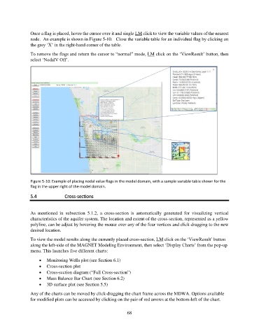
Once a flag is placed, hover the cursor over it and single LM click to view the variable values of the nearest
node. An example is shown in Figure 5-10. Close the variable table for an individual flag by clicking on
the grey ‘X’ in the right-hand corner of the table.

To remove the flags and return the cursor to “normal” mode, LM click on the ‘ViewResult’ button, then
select ‘NodalV Off’.

Figure 5-10: Example of placing nodal value flags in the model domain, with a sample variable table shown for the
flag in the upper right of the model domain.

5.4 Cross-sections

As mentioned in subsection 5.1.2, a cross-section is automatically generated for visualizing vertical
characteristics of the aquifer system. The location and extent of the cross-section, represented as a yellow
polyline, can be adjust by hovering the mouse over any of the four vertices and click-dragging to the new
desired location.

To view the model results along the currently placed cross-section, LM click on the ‘ViewResult’ button
along the left-side of the MAGNET Modeling Environment, then select ‘Display Charts’ from the pop-up
menu. This launches five different charts:

• Monitoring Wells plot (see Section 6.1)
• Cross-section plot
• Cross-section diagram (“Full Cross-section”)
• Mass Balance Bar Chart (see Section 6.2)
• 3D surface plot (see Section 5.5)

Any of the charts can be moved by click-dragging the chart frame across the MDWA. Options available
for modified plots can be accessed by clicking on the pair of red arrows at the bottom-left of the chart.

68