Page 49 - ansys

It can also be used in cases where there is discontinuity in the flow where FDM fails to calculate.
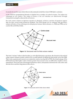
In the FVM the computational domain is divided into a number of control volumes. The values are
calculated at cell centers. The values of fluxes at the cell interface are determined through
interpolation using the values at the cell centers.
For each control volume an algebraic equation is obtained, and thus a number of equations appear
that are then solved using numerical methods. The FVM should not be confused with geometric
volume definition. It has nothing to do with physical volume. Both schemes, i.e., FDM and FVM, can be
used in 2D and 3D flow fields.

The term “volume” refers to the fact that, to solve fluid dynamics equations, the domain is discretized
using control volumes (which could be 2D, as well) instead of taking discrete points as for the FDM.
This is also a paramount reason to accommodate unstructured grids in FVM. One disadvantage of the
FVM method is that higher-order schemes greater than second order are difficult to handle in three
dimensions. This is because of dual approximations: that is, interpolation between the cell centers and
the interfaces and the integration of all surfaces.

42