Page 412 - Adams and Stashak's Lameness in Horses, 7th Edition

378 Chapter 3

VetBooks.ir

A B
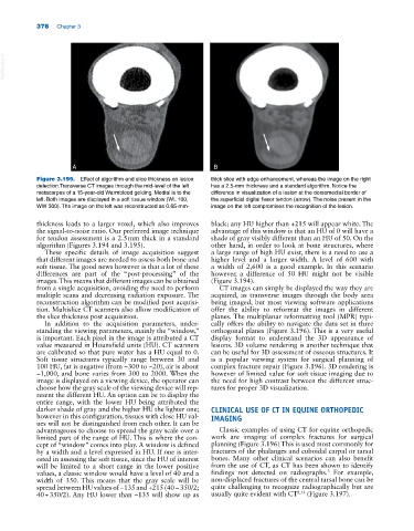
Figure 3.195. Effect of algorithm and slice thickness on lesion thick slice with edge enhancement, whereas the image on the right
detection.Transverse CT images through the mid‐level of the left has a 2.5‐mm thickness and a standard algorithm. Notice the
metacarpus of a 15‐year‐old Warmblood gelding. Medial is to the difference in visualization of a lesion at the dorsomedial border of
left. Both images are displayed in a soft tissue window (WL 100, the superficial digital flexor tendon (arrow). The noise present in the
WW 300). The image on the left was reconstructed as 0.65‐mm‐ image on the left compromises the recognition of the lesion.

thickness leads to a larger voxel, which also improves black; any HU higher than +215 will appear white. The
the signal‐to‐noise ratio. Our preferred image technique advantage of this window is that an HU of 0 will have a
for tendon assessment is a 2.5 mm thick in a standard shade of gray visibly different than an HU of 50. On the
algorithm (Figures 3.194 and 3.195). other hand, in order to look at bone structures, where
These specific details of image acquisition suggest a large range of high HU exist, there is a need to use a
that different images are needed to assess both bone and higher level and a larger width. A level of 600 with
soft tissue. The good news however is that a lot of these a width of 2,600 is a good example. In this scenario
differences are part of the “post‐processing” of the however, a difference of 50 HU might not be visible
images. This means that different images can be obtained (Figure 3.194).
from a single acquisition, avoiding the need to perform CT images can simply be displayed the way they are
multiple scans and decreasing radiation exposure. The acquired, as transverse images through the body area
reconstruction algorithm can be modified post acquisi­ being imaged, but most viewing software applications
tion. Multislice CT scanners also allow modification of offer the ability to reformat the images in different
the slice thickness post acquisition. planes. The multiplanar reformatting tool (MPR) typi­
In addition to the acquisition parameters, under­ cally offers the ability to navigate the data set in three
standing the viewing parameters, mainly the “window,” orthogonal planes (Figure 3.196). This is a very useful
is important. Each pixel in the image is attributed a CT display format to understand the 3D appearance of
value measured in Hounsfield units (HU). CT scanners lesions. 3D volume rendering is another technique that
are calibrated so that pure water has a HU equal to 0. can be useful for 3D assessment of osseous structures. It
Soft tissue structures typically range between 30 and is a popular viewing system for surgical planning of
100 HU, fat is negative (from −300 to −20), air is about complex fracture repair (Figure 3.196). 3D rendering is
−1,000, and bone varies from 300 to 2000. When the however of limited value for soft tissue imaging due to
image is displayed on a viewing device, the operator can the need for high contrast between the different struc­
choose how the gray scale of the viewing device will rep­ tures for proper 3D visualization.
resent the different HU. An option can be to display the
entire range, with the lower HU being attributed the
darker shade of gray and the higher HU the lighter one; CLINICAL USE OF CT IN EQUINE ORTHOPEDIC
however in this configuration, tissues with close HU val­ IMAGING
ues will not be distinguished from each other. It can be
advantageous to choose to spread the gray scale over a Classic examples of using CT for equine orthopedic
limited part of the range of HU. This is where the con­ work are imaging of complex fractures for surgical
cept of “window” comes into play. A window is defined planning (Figure 3.196) This is used most commonly for
by a width and a level expressed in HU. If one is inter­ fractures of the phalanges and cuboidal carpal or tarsal
ested in assessing the soft tissue, since the HU of interest bones. Many other clinical scenarios can also benefit
will be limited to a short range in the lower positive from the use of CT, as CT has been shown to identify
3
values, a classic window would have a level of 40 and a findings not detected on radiographs. For example,
width of 350. This means that the gray scale will be non‐displaced fractures of the central tarsal bone can be
spread between HU values of −135 and +215 (40 – 350/2; quite challenging to recognize radiographically but are
40 + 350/2). Any HU lower than −135 will show up as usually quite evident with CT 8,13 (Figure 3.197).