Page 411 - Adams and Stashak's Lameness in Horses, 7th Edition

Diagnostic Imaging 377

VetBooks.ir

0.65 mm thick 0.65 mm thick 2.5 mm thick
edge enhancement standard algorithm standard algorithm

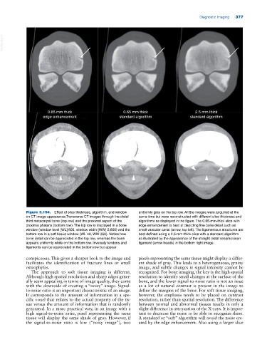
Figure 3.194. Effect of slice thickness, algorithm, and window uniformly gray on the top row. All the images were acquired at the
on CT image appearance.Transverse CT images through the distal same time but were reconstructed with different slice thickness and
third metacarpal bone (top row) and the proximal aspect of the algorithms as displayed in the figure. The 0.65‐mm‐thick slice with
proximal phalanx (bottom row). The top row is displayed in a bone edge enhancement is best at depicting fine bone detail such as
window (window level [WL] 600, window width [WW] 2,600) and the small vascular canal (arrow, top left). The ligamentous structures are
bottom row in a soft tissue window (WL 40, WW 350). Notice how best defined using a 2.5‐mm‐thick slice with a standard algorithm
bone detail can be appreciated in the top row, whereas the bone as illustrated by the appearance of the straight distal sesamoidean
appears uniformly white on the bottom row. Inversely tendons and ligament (arrow heads) in the bottom right image.
ligaments can be appreciated in the bottom row but appear

conspicuous. This gives a sharper look to the image and pixels representing the same tissue might display a differ­
facilitates the identification of fracture lines or small ent shade of gray. This leads to a heterogeneous, grainy
osteophytes. image, and subtle changes in signal intensity cannot be
The approach to soft tissue imaging is different. recognized. For bone imaging, the key is the high spatial
Although high spatial resolution and sharp edges gener­ resolution to identify small changes at the surface of the
ally seem appealing in terms of image quality, they come bone, and the lower signal‐to‐noise ratio is not an issue
with the downside of creating a “noisy” image. Signal‐ as a lot of natural contrast is present in the image to
to‐noise ratio is an important characteristic of an image. define the margins of the bone. For soft tissue imaging,
It corresponds to the amount of information in a spe­ however, the emphasis needs to be placed on contrast
cific voxel that relates to the actual property of the tis­ resolution, rather than spatial resolution. The difference
sue versus the amount of information that is randomly between normal and abnormal tissues results in only a
generated. In a more practical way, in an image with a slight difference in attenuation of the X‐rays. It is impor­
high signal‐to‐noise ratio, pixel representing the same tant to decrease the noise to be able to recognize these.
tissue will display the same shade of gray. However, if A standard or “soft” algorithm will avoid the noise cre­
the signal‐to‐noise ratio is low (“noisy image”), two ated by the edge enhancement. Also using a larger slice