Page 4 - Cutting tool temperature prediction method using analytical model for end milling

Cutting tool temperature prediction method using analytical model for end milling 1791

2 Z x t 2
erfðxÞ¼ p ffiffiffi e dt ð8Þ
p 0
Then GU which represents the integral of variable x is cal-
culated as
" ! !#
Z 2 2
L x ðx þ x p Þ ðx x p Þ
GUðx; L x ; DÞ¼ exp 2 þ exp 2 dx p
0 D D
p ffiffiffi " Z xþLx Z x #
p 2 D t 2 D t 2
¼ D p e dt e dt
ffiffiffi
2 p x xLx
D D
p ffiffiffi
p x þ L x x L x
¼ D erf þ erf ð9Þ
2 D D
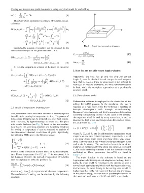
Fig. 3 Insert heat convection diagram.
Similarly, the integral of variable y can be obtained. So the
inner double integral of the green function GR is
2 sin l n
C n ¼ ð15Þ

2 z 2 l þ cos l sin l n

n
n
GRðx; y; z; L x ; L y ; DÞ¼ p ffiffiffi 3 exp 2
ðD pÞ D
hL
n
GUðx; L x ; DÞGUðx; L y ; DÞ ð10Þ tan l ¼ ð16Þ
kl n
At last, the temperature solution of the insert on the cutter
is 3. Heat flux and tool-chip contact length evaluation
Z t
a
Tðx; y; z; tÞ¼ GRðx; y; z; b; L x ; L y ; DÞqðsÞds
k 0 Apparently, the heat flux Q and the chip-tool contact
Z t 2 length L x must be obtained in order to get the tool tempera-
a 1 z
þ p ffiffiffi exp GLðx; L x ; b; DÞ ture. But to measure them by experiment is too difficult to
0 2D p D 2
k
realize; as an effective alternative, the finite element simulation
ð11Þ
GUðy; L y ; DÞqðsÞds
is fixed, while the workpiece approaches at a particularly
where constant speed.
1 x
GLðx; L x ; b; DÞ¼ 1 ðGUðx; L x ; DÞ 3.1. Finite element model
L x
1 b
GUðx; b; L x ; DÞÞ ð12Þ
Deformation software is employed in the simulation of the
milling Inconel718 process. In the simulation, the tool is
regarded as a rigid body, while the workpiece is regarded as
2.2. Model of temperature dropping phase
isotropic elastic–plastic with isotropic strain-hardening.
Because of high strain rate and high temperature deformation
This phase refers to the time when the insert is entirely exposed
occurring in machining Inconel718, the Jason-Cook constitu-
in ambient air, causing its temperature to drop. The process of tive equation, which is used by many researchers, is used to
temperature dropping can be modeled as one of heat convec- describe the high strain and temperature deformation behav-
tion. Therefore, by approximating the insert as a thin plate ior, as given in Eq. (17):
with certain thickness (see Fig. 3), based on the heat conduc-
m
tion theory, the governing equation and boundary condition n T d T r
e ¼ðA þ B e Þð1 þ C ln _ eÞ 1 ð17Þ
for solving its temperature T can be obtained by analysis of T m T r
one-dimensional thermal conduction of plate. Specifically, where T d , T r , and T m are the deformation temperature, room
the following PDEs are in the following order:
temperature and melt point temperature, respectively. e, e and
8 2 _ e are shear stress, shear strain and shear strain rate, respec-
@T @ T
@t
> ¼ a @z 2
>
< tively. The constants A and B stand for the material yield stress
@Tðz;sÞ ¼ 0 z ¼ 0 ð13Þ
@z and strain hardening. The mechanics characteristics of the
>
>
: @Tðz;sÞ ¼ hðTðL; sÞ T f Þ z ¼ L material are represented by the stress rate sensitive coefficient
@z
k
C, the strain hardening exponent n and the thermal softening
where h is the convection transfer rate and T f fluid tempera- coefficient m. These parameters Inconel718 are listed in
ture. Excess temperature h ¼ TðL; sÞ T f is introduced, L is Table 1. 19
the thickness of insert, the method of separation of variables The mesh function in the software is based on the
then be employed to solve the problem, i.e. Lagrangian-Euler techniques and adaptive re-meshing. Specif-
1 ically, the mesh could be remeshed in the vicinity to form a
hðg; sÞ X 2
¼ C n exp l F 0 cosðl gÞ ð14Þ normal mesh again after the initial mesh has become distorted.
n n
h 0
n¼1 Furthermore, the mesh density in the cutting zone should be
x higher than that in the rest regions of the tool and workpiece.
where g ¼ , F 0 ¼ as 2 , h 0 represents initial excess temperature.
L L
The coefficients C n and l can be obtained by the following In the present study, the numbers of quadrangle elements in
n
equation: the insert and workpiece are 28197 and 49079 respectively.