Page 5 - Cutting tool temperature prediction method using analytical model for end milling

1792 W. Baohai et al.

Table 1 Jason-cook constitutive of Table 3 Fitting formula of chip-tool contact length.
Inconel718 parameters.
Cutting Fitting polynomial
Parameter Value speed
(m/min)
A (MPa) 450
9
9
2
B (MPa) 1700 60 L x ¼2:089 10 f þ 1:588 10 f z þ 4:677 10 7
z
9
2
9
C 0.017 80 L x ¼1:018 10 f þ 1:373 10 f z þ 6:168 10 7
z
m 1.3 100 L x ¼1:429 10 f þ 1:078 10 f z þ 7:686 10 7
9
2
8
n 0.65 z
T r (°C) 20
T m (°C) 1590
Table 4 Fitting formula of heat flux.
The simulation is performed at ambient temperature pro-
Cutting Fitting polynomial
vided that the initial temperature of the tool and workpiece
speed (m/
is 20 °C. The convection coefficient between the workpiece
min)
and air is set as 20 W=ðm CÞ. According to the Coulomb 11 2 11 9
2
law, the friction factor is taken to be 0.4. During the simula- 60 q ¼ 1:25 10 f þ 1:21 10 f z 6:64 10
z
2
10
10
tion, the insert rake angle 5° and clearance angle 5° are fixed, 80 q ¼ 1:79 10 f 8:48 10 f z 3:84 10 9
z
2
10
10
while the workpiece approaches at a particularly constant 100 q ¼ 7:14 10 f þ 6:21 10 f z 3:88 10 8
z
speed.
3.2. Chip-tool contact length L x evaluation
in the chip-tool interface can reach the tool. 20 Equation below
The whole simulation is divided into three groups based on the provides a way to calculate it:
cutting speed, i.e., the cutting speed V is 60 m/min, 80 m/min,
p ffiffiffiffiffiffiffiffiffiffiffiffi
and 100 m/min. At each of the three, the simulation is per- k t q c t
t
c ¼ p ffiffiffiffiffiffiffiffi p ffiffiffiffiffiffiffiffiffiffiffiffi ð18Þ
formed by altering feed per tooth f in the range from kqc þ k t q c t
z
t
0.12 mm/z to 0.20 mm/z. The radial depth of cut a e and axial
where k, q and c respectively represent thermal conductivity,
depth of cut a p are set to be 4 mm and 0.5 mm respectively.
density, and specific heat, with the subscript t indicating
The fitting formula about the relationship between L x and f z
at any particular cutting speed is obtained by the least- whether the particular coefficient is for the tool (with t) or
the workpiece (without t). The specific results of the heat flux
square curve fitting method. The specific results from the sim-
Q and the fitting formulas are listed in Table 4.
ulation and the fitting formulas are listed in Tables 2 and 3.
3.3. Heat flux evaluation 4. Experiments
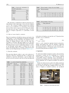
The same finite element method is used in the evaluation of To verify the established temperature model, a physical milling
heat flux Q. However, compared with the L x evaluation, the experiment is carried out. It is performed at a four-axis
machine center, as shown in Fig. 4. The workpiece material
coefficient of heat flux distribution c must be taken into
is Inconel718, which is extensively used in aeroengines. A
account in the Q evaluation, since not all heat flux generated
double-tooth end milling cutter with a carbide insert is selected
in this experiment and its specific parameters are shown in
Table 2 L x and Q obtained from simulation. Table 5.
Single wire thermocouple is used in the milling experiment
Cutting speed Feed per The chip-tool Heat flux to measure the temperature. First, the workpiece is divided
(m/min) tooth (mm/z) contact length (m) (W=m )
2
into two parts across the line of milling direction. Next, two
60 0.12 206.7 10 6 6.2 10 9 pieces of megahit, as insulted conductor, are introduced
0.14 229.4 10 6 7.8 10 9
0.16 246.9 10 6 8.9 10 9
0.18 264.3 10 6 11.7 10 9
0.20 281.2 10 6 12.2 10 9
80 0.12 213.0 10 6 6.7 10 9
0.14 230.2 10 6 8.2 10 9
0.16 259.5 10 6 10.1 10 9
0.18 274.1 10 6 12.3 10 9
0.20 295.8 10 6 13.7 10 9
100 0.12 204.8 10 6 8.1 10 9
0.14 224.3 10 6 9.7 10 9
0.16 243.5 10 6 11.4 10 9
0.18 269.7 10 6 13.1 10 9
0.20 285.3 10 6 14.9 10 9
Fig. 4 Temperature measuring experiment.