Page 243 - Six Sigma Advanced Tools for Black Belts and Master Black Belts

OTE/SPH
OTE/SPH
August 31, 2006
3:4
Char Count= 0
JWBK119-15
228 Development of A Moisture Soak Model For Surface Mounted Devices
0.350
0.300 (a)
0.250
% Weight Gain (%) 0.200 (b)

(c)
0.150

0.100
(d)
0.050
Time Duration (hours)
0.000
0 20 40 60 80 100 120 140 160 180 200

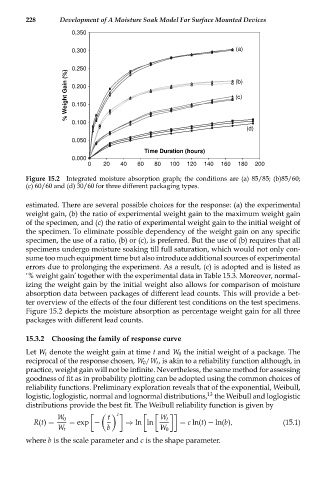
Figure 15.2 Integrated moisture absorption graph; the conditions are (a) 85/85; (b)85/60;
(c) 60/60 and (d) 30/60 for three different packaging types.

estimated. There are several possible choices for the response: (a) the experimental
weight gain, (b) the ratio of experimental weight gain to the maximum weight gain
of the specimen, and (c) the ratio of experimental weight gain to the initial weight of
the specimen. To eliminate possible dependency of the weight gain on any specific
specimen, the use of a ratio, (b) or (c), is preferred. But the use of (b) requires that all
specimens undergo moisture soaking till full saturation, which would not only con-
sume too much equipment time but also introduce additional sources of experimental
errors due to prolonging the experiment. As a result, (c) is adopted and is listed as
‘% weight gain’ together with the experimental data in Table 15.3. Moreover, normal-
izing the weight gain by the initial weight also allows for comparison of moisture
absorption data between packages of different lead counts. This will provide a bet-
ter overview of the effects of the four different test conditions on the test specimens.
Figure 15.2 depicts the moisture absorption as percentage weight gain for all three
packages with different lead counts.

15.3.2 Choosing the family of response curve
Let W t denote the weight gain at time t and W 0 the initial weight of a package. The
reciprocal of the response chosen, W 0 /W t , is akin to a reliability function although, in
practice, weight gain will not be infinite. Nevertheless, the same method for assessing
goodness of fit as in probability plotting can be adopted using the common choices of
reliability functions. Preliminary exploration reveals that of the exponential, Weibull,
13
logistic, loglogistic, normal and lognormal distributions, the Weibull and loglogistic
distributions provide the best fit. The Weibull reliability function is given by
c

W 0 t W t
R(t) = = exp − ⇒ ln ln = c ln(t) − ln(b), (15.1)
W t b W 0
where b is the scale parameter and c is the shape parameter.