Page 246 - Six Sigma Advanced Tools for Black Belts and Master Black Belts

OTE/SPH
OTE/SPH
Char Count= 0
August 31, 2006
3:4
JWBK119-15
Moisture Soak Model 231
In general, one could express the location parameter as a linear function of ln(T),
1/T, RH, ln(RH), RH/T or other similar independent variables which are variants of
the above forms. This results in
1 RH

a = f , RH, ln(T) ln(RH), . (15.9)
T T
Here we adopt a ‘combined’ analysis given that the loglogistic distribution function
provides the best fit. From equation (15.2), we have

W t − W 0
a =−b ln + ln(t). (15.10)
W 0
It follows that the generic form is

W t − W 0 1 RH
ln = α 0 + α 1 ln(t) + f , RH, ln(T), , ln(RH) . (15.11)
W 0 kT T
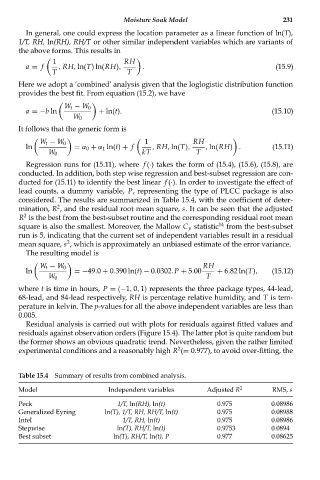
Regression runs for (15.11), where f (·) takes the form of (15.4), (15.6), (15.8), are
conducted. In addition, both step wise regression and best-subset regression are con-
ducted for (15.11) to identify the best linear f (·). In order to investigate the effect of
lead counts, a dummy variable, P, representing the type of PLCC package is also
considered. The results are summarized in Table 15.4, with the coefficient of deter-
2
mination, R , and the residual root mean square, s. It can be seen that the adjusted
2
R is the best from the best-subset routine and the corresponding residual root mean
square is also the smallest. Moreover, the Mallow C p statistic 14 from the best-subset
run is 5, indicating that the current set of independent variables result in a residual
2
mean square, s , which is approximately an unbiased estimate of the error variance.
The resulting model is

W t − W 0 RH
ln =−49.0 + 0.390 ln(t) − 0.0302.P + 5.00 + 6.82 ln(T), (15.12)
W 0 T
where t is time in hours, P = (−1, 0, 1) represents the three package types, 44-lead,
68-lead, and 84-lead respectively, RH is percentage relative humidity, and T is tem-
perature in kelvin. The p-values for all the above independent variables are less than
0.005.
Residual analysis is carried out with plots for residuals against fitted values and
residuals against observation orders (Figure 15.4). The latter plot is quite random but
the former shows an obvious quadratic trend. Nevertheless, given the rather limited
2
experimental conditions and a reasonably high R (= 0.977), to avoid over-fitting, the

Table 15.4 Summary of results from combined analysis.
Model Independent variables Adjusted R 2 RMS, s

Peck 1/T, ln(RH), ln(t) 0.975 0.08986
Generalized Eyring ln(T), 1/T, RH, RH/T, ln(t) 0.975 0.08988
Intel 1/T, RH, ln(t) 0.975 0.08986
Stepwise ln(T), RH/T, ln(t) 0.9753 0.0894
Best subset ln(T), RH/T, ln(t), P 0.977 0.08625