Page 244 - Six Sigma Advanced Tools for Black Belts and Master Black Belts

OTE/SPH
OTE/SPH
August 31, 2006
3:4
Char Count= 0
JWBK119-15
Moisture Soak Model 229
The loglogistic reliability function is given by
W 0 exp [− (ln(t) − a) /b] W t − W 0 ln(t) − a
R(t) = = ⇒ ln = , (15.2)
W t 1 + exp [− (ln(t) − a) /b] W 0 b
where a is the location parameter and b is the scale parameter. The good fit to both
distributions is expected as, when W t − W 0 is small, we have

W t W t − W 0
ln ≈ .
W 0 W 0
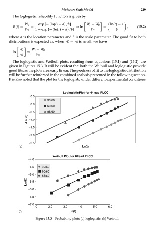
The loglogistic and Weibull plots, resulting from equations (15.1) and (15.2), are
given in Figures 15.3. It will be evident that both the Weibull and loglogistic provide
goodfits,astheplotsarenearlylinear.Thegoodnessoffittotheloglogisticdistribution
will be further reinforced in the combined analysis presented in the following section.
It is also noted that the plot for the loglogistic under different experimental conditions

Loglogistic Plot for 44lead PLCC
0.5
30/60
0.0
60/60
−0.5 85/60
-LnH(t) −1.0

−1.5

−2.0
−2.5
(a) Ln(t)

Weibull Plot for 84lead PLCC
−4.0
−4.5 30/60
60/60
−5.0
85/60
LnH(t) −5.5

−6.0
−6.5

−7.0
1.0 2.0 3.0 4.0 5.0 6.0
(b) Ln(t)

Figure 15.3 Probability plots: (a) loglogistic; (b) Weibull.