Page 316 - Six Sigma Advanced Tools for Black Belts and Master Black Belts

OTE/SPH
OTE/SPH
3:6
Char Count= 0
August 31, 2006
JWBK119-19
Potential of Lean Design 301
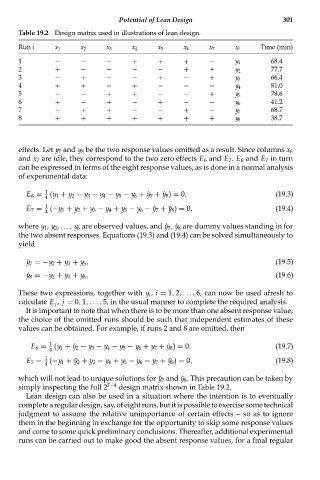
Table 19.2 Design matrix used in illustrations of lean design.
Run i x 1 x 2 x 3 x 4 x 5 x 6 x 7 x i Time (min)
1 − − − + + + − y 1 68.4
2 + − − − − + + y 2 77.7
3 − + − − + − + y 3 66.4
4 + + − + − − − y 4 81.0
5 − − + + − − + y 5 78.6
6 + − + − + − − y 6 41.2
7 − + + − − + − y 7 68.7
8 + + + + + + + y 8 38.7

effects. Let y 7 and y 8 be the two response values omitted as a result. Since columns x 6
and x 7 are idle, they correspond to the two zero effects E 6 and E 7 . E 6 and E 7 in turn
can be expressed in terms of the eight response values, as is done in a normal analysis
of experimental data:

1
E 6 = (y 1 + y 2 − y 3 − y 4 − y 5 − y 6 + ˆy 7 + ˆy 8 ) = 0, (19.3)
4
1
E 7 = (−y 1 + y 2 + y 3 − y 4 + y 5 − y 6 − ˆy 7 + ˆy 8 ) = 0, (19.4)
4
where y 1 , y 2 ,. . . , y 6 are observed values, and ˆy 7 , ˆy 8 are dummy values standing in for
the two absent responses. Equations (19.3) and (19.4) can be solved simultaneously to
yield

ˆ y 7 =−y 2 + y 3 + y 5 , (19.5)
ˆ y 8 =−y 2 + y 4 + y 6 . (19.6)

These two expressions, together with y i , i = 1, 2,..., 6, can now be used afresh to
calculate E j , j = 0, 1,..., 5, in the usual manner to complete the required analysis.
It is important to note that when there is to be more than one absent response value,
the choice of the omitted runs should be such that independent estimates of these
values can be obtained. For example, if runs 2 and 8 are omitted, then

1
E 6 = (y 1 + ˆy 2 − y 3 − y 4 − y 5 − y 6 + y 7 + ˆy 8 ) = 0, (19.7)
4
1
E 7 = (−y 1 + ˆy 2 + y 3 − y 4 + y 5 − y 6 − y 7 + ˆy 8 ) = 0, (19.8)
4
which will not lead to unique solutions for ˆy 2 and ˆy 8 . This precaution can be taken by
simply inspecting the full 2 7−4 design matrix shown in Table 19.2.
Lean design can also be used in a situation where the intention is to eventually
completearegulardesign,say,ofeightruns,butitispossibletoexercisesometechnical
judgment to assume the relative unimportance of certain effects -- so as to ignore
them in the beginning in exchange for the opportunity to skip some response values
and come to some quick preliminary conclusions. Thereafter, additional experimental
runs can be carried out to make good the absent response values, for a final regular