Page 327 - Six Sigma Advanced Tools for Black Belts and Master Black Belts

OTE/SPH
OTE/SPH
Char Count= 0
August 31, 2006
JWBK119-20
3:6
312 A Unified Approach for Dual Response Surface Optimization
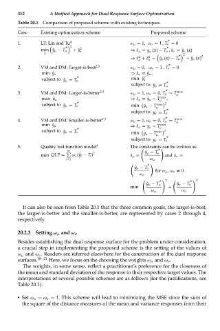
Table 20.1 Comparison of proposed scheme with existing techniques.
Case Existing optimization scheme Proposed scheme
*
1. LT: Lin and Tu 4 ω μ = 1, ω σ = 1 , T σ = 0
2
* 2 *

min ˆy μ − T μ + ˆy σ ⇒ δ μ = y μ (x) − T μ ,δ σ = ˆy σ (x)
X
2
2 2 * 2
⇒ δ + δ = ˆy u (x) − T μ + ˆy σ (x)
μ
σ
*
2. VM and DM: Target-is-best 2,3 ω μ = 0, ω σ = 1 , T σ = 0
min ˆy σ ⇒ δ σ = ˆy σ ,
* min ˆy 2
subject to ˆy μ = T μ σ
*
subject to ˆy μ = T μ
*
3. VM and DM: Larger-is-better 2,3 ω μ = 1,ω σ = 0, T μ = T μ max
⇒ δ μ = ˆy μ − T max ,
max ˆy μ μ
* max 2
ˆ
subject to ˆy σ = T σ min y μ − T μ
*
subject to y σ = T σ
*
4. VM and DM: Smaller-is-better 2,3 ω μ = 1,ω σ = 0, T μ = T min
μ
min ˆy μ ⇒ δ μ = y μ − T min
* μ 2
min y μ − T
subject to ˆy σ = T σ min
μ
*
subject to y σ = T σ
5. Quality lost function model 6 The constraints can be written as
*

m
min QLP = ω i ( ˆy i − T i ) 2 δ μ = ˆ y μ − T μ and δ σ =
i=1 ω μ
*

ˆ y σ − T σ
for ω μ ,ω σ = 0
ω σ
* *

2
2
ˆ y μ − T μ ˆ y σ − T σ
min +
ω μ ω σ
It can also be seen from Table 20.1 that the three common goals, the target-is-best,
the larger-is-better and the smaller-is-better, are represented by cases 2 through 4,
respectively.
20.2.3 Setting ω μ and ω σ
Besides establishing the dual response surface for the problem under consideration,
a crucial step in implementing the proposed scheme is the setting of the values of
ω μ and ω σ . Readers are referred elsewhere for the construction of the dual response
surfaces. 18−21 Here, we focus on the choosing the weights ω μ and ω σ .
The weights, in some sense, reflect a practitioner’s preference for the closeness of
the mean and standard deviation of the response to their respective target values. The
interpretations of several possible schemes are as follows (for the justifications, see
Table 20.1).
Set ω μ = ω σ = 1. This scheme will lead to minimizing the MSE since the sum of
the square of the distance measures of the mean and variance responses from their