Page 330 - Six Sigma Advanced Tools for Black Belts and Master Black Belts

OTE/SPH
OTE/SPH
August 31, 2006
Char Count= 0
JWBK119-20
3:6
Example 1 315
T
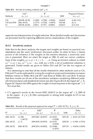
Table 20.3 Results of existing methods (xx ≤ 3).
Y(x) T X T Proposed Scheme
Methods (γ μ ,γ σ ) (x 1 , x 2 , x 3 ) MSE (ω μ ,ω σ )
CN (495.88, 40.22) (1.5683, −0.7290, −0.0946) 1634.68 (0.49, 0.51)
VM and DM (500, 40.65) (1.5719, −0.7220, −0.0874) 1652.46 (0, 1)
LT (495.68, 40.20) (15651, −0.7373, −0.0883) 1634.57 (0.5, 0.5)

supports our interpretation of weight selection. More detailed results and discussions
are presented next by exploring different convex combinations of the weights.

20.3.2 Sensitivity analysis
Note that in the above analysis, the targets and weights are based on practical con-
siderations and the users’ preferences discussed earlier. In order to have a clearer
picture of the influence of the weights on the solution obtained, a sensitivity anal-
ysis is presented. Here we select the target as (500, 0) and use convex combina-
j j
tions of the weights, ω μ + ω σ = 1, j = 1,. . . , m. Using an iterative scheme in which
j+1 j j+1 j
ω μ = ω μ + ω, ω σ = ω σ − ω, with ω = 0.01, a set of noninferior solutions is
generated. Partial results are given in Tables 20.6 and 20.7 for the two regions of
interest.
It is interesting to note that all the results obtained by other methods such as CN,
DM and LT can be replicated by tuning the weights in proposed formulation (compare
boldface entries in Tables 20.6 and 20.7 and those in Tables 20.3 and 20.5). It means
that these results are all one of the noninferior solutions considering different trade-
T
offs between mean and standard deviation (see also Figure 20.2 in the region xx ≤ 3).
T
Figure 20.3 depicts the MSE against the weight of mean response in the region xx ≤ 3.
It is clear that

T
LT’s approach results in the lowest MSE (1634.57 in the region xx ≤ 3; 2005.14
in the region −1 ≤ x ≤ 1) (this corresponds to setting both weights to 0.5 in our
formulation);

Table 20.4 Results of the proposed approach for target T* = (500, 44.72) (−1 ≤ x ≤ 1).
ω Y(X) T X T Delta
T* (ω μ ,ω σ ) (y μ , y σ ) (x 1 , x 2 , x 3 ) MSE (δ μ ,δ σ )

(500, 44.72) (1/500, (499.9667, 45.0937) (1,0.1183, 2033.44 (−16.65, 16.7119)
1/44.72) −0.2598)
(500, 44.72) (1, 1) (499.6639, 45.0574) (1,0.1157, 2030.29 (−0.3361, 0.3374)
−0.2593)
(500, 44.72) (500, 44.72) (498.2014, 44.8822) (1,0.1040, 2017.65 (−0.0036, 0.0036)
−0.2575)