Page 333 - Six Sigma Advanced Tools for Black Belts and Master Black Belts

OTE/SPH
OTE/SPH
August 31, 2006
3:6
Char Count= 0
JWBK119-20
318 A Unified Approach for Dual Response Surface Optimization
CN’s approach does minimize the variance response while allowing the deviation
of mean value from the target within a interval; (The result can be closely replicated
T
by setting ω μ = 0.49,ω σ = 0.51 in proposed scheme for xx ≤ 3);
KL’s approach results in maximum degree of satisfaction in terms of the membership
function constructed (the result can be closely replicated by setting ω μ = 0.46,ω σ =
0.54 in the proposed scheme for −1 ≤ x ≤ 1);
VM and DM’s approach gives the minimum variance while keeping the mean at a
specified target value (500) (this corresponds to setting the weights to (0, 1) in the
proposed scheme).

*
From the sensitivity analysis, the effect of the weights on how near ˆy μ (x) is to T μ
*
and how near ˆy σ (x)isto T σ can easily be inferred. For example, when the weight
of the mean response increases, the deviation from the mean target increases while
the deviation from the variance response target decreases. This is shown clearly in
Figure 20.2. Moreover, for the problem considered, the deviation between the mean
targets and the proposed solution increases rapidly when ω μ is increased beyond 0.6.
In Figure 20.3, it is observed that there is an optimal weight combination (when both
weights are 0.5) that will result in minimum MSE, which is identical to the objective
of LT’s approach.

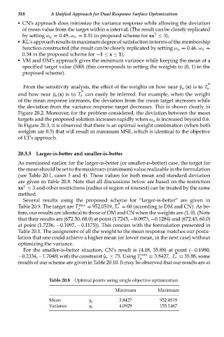
20.3.3 Larger-is-better and smaller-is-better

As mentioned earlier, for the larger-is-better (or smaller-is-better) case, the target for
themeanshouldbesettothemaximum(minimum)valuerealizableintheformulation
(see Table 20.1, cases 3 and 4). These values for both mean and standard deviation
are given in Table 20.8. Note that all discussions below are based on the restriction
T
xx ≤ 3 and other restrictions (radius of region of interest) can be treated by the same
method.
Several results using the proposed scheme for “larger-is-better’’ are given in
*
Table 20.9. The target are T max = 952.0519, T σ = 60 (according to DM and CN). As be-
μ
fore, our results are identical to those of DM and CN when the weights are (1, 0). (Note
that their results are (672.50, 60.0) at point (1.7245, −0.0973, −0.1284) and (672.43, 60.0)
at point (1.7236, −0.1097, −0.1175)). This concurs with the formulation presented in
Table 20.1. The assignment of all the weight to the mean response matches our postu-
lation that one could achieve a higher mean (or lower mean, in the next case) without
optimizing the variance.
For the smaller-is-better situation, CN’s result is (4.18, 35.88) at point (−0.1980,
*
−0.2334, −1.7048) with the constraint ˆy σ ≤ 75. Using T min = 3.8427, T σ = 35.88, some
μ
results of our scheme are given in Table 20.10. It may be observed that our results are at

Table 20.8 Optimal points using single objective optimization.
Minimum Maximum

Mean y μ 3.8427 952.0519
Variance y σ 4.0929 155.1467