Page 329 - Six Sigma Advanced Tools for Black Belts and Master Black Belts

OTE/SPH
OTE/SPH
Char Count= 0
August 31, 2006
JWBK119-20
3:6
314 A Unified Approach for Dual Response Surface Optimization
20.3 EXAMPLE 1
In this section, we compare various solutions from our formulation with other results
using a classical example of a printing process. This example is taken from Box and
18
Draper, anditisalsousedelsewhere. 2−5,7 Thepurposeoftheexperimentistoanalyze
the effect of the speed, pressure, and distance variables on the ability that a printing
machine has for applying colored ink to package labels. The proposed fitted response
surface for the mean and standard deviation of the characteristic of interest are as
follows: 2

2 2 2
ˆ y μ = 327.6 + 177.0x 1 + 109.4x 2 + 131.5x 3 + 32.0x − 22.4x − 29.1x + 66.0x 1 x 2
1 2 3
+ 75.5x 1 x 3 + 43.6x 2 x 3 ,
2 2 2
y σ = 34.9 + 11.5x 1 + 15.3x 2 + 29.2x 3 + 4.2x − 1.3x + 16.8x + 7.7x 1 x 2
1 2 3
+5.1x 1 x 3 + 14.1x 2 x 3 .

20.3.1 Target-is-best
We consider two cases with the target for the mean at 500, with different targets for
the standard deviation at 40 and 44.72.

T
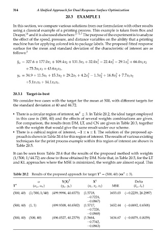
There is a circular region of interest, xx ≤ 3. In Table 20.2, the ideal target employed
in this case is (500, 40) and the effects of several weights combinations are given.
For comparison, the results from DM, LT, and CN are given in Table 20.3, together
with the weights that would give the same result under our scheme.
There is a cubical region of interest, −1 ≤ x ≤ 1. The solution of the proposed ap-
proach is shown in Table 20.4 for this region of interest. The results of various existing
techniques for the print process example within this region of interest are shown in
Table 20.5.
It can be seen from Table 20.4 that the results of the proposed method with weights
(1/500, 1/44.72) are close to those obtained by DM. Note that, in Table 20.5, for the LT
and KL approaches where the MSE is minimized, the weights are almost equal. This

T
Table 20.2 Results of the proposed approach for target T* = (500, 40) (xx ≤ 3).
ω Y(X) T X T Delta
T* (ω μ ,ω σ ) (y μ , y σ ) (x 1 , x 2 , x 3 ) MSE (δ μ ,δ σ )

(500, 40) (1/500,1/40) (499.9996, 40.6575) (1.5718, 1653.03 (−0.2239, 26.2987)
−0.7224,
−0.0867)
(500, 40) (1, 1) (499.9308, 40.6502) (1.5717, 1652.44 (−0.0692, 0.6501)
−0.7226,
−0.0868)
(500, 40) (500, 40) (496.0527, 40.2379) (1.5664, 1634.67 (−0.0079, 0.0059)
−0.7342,
−0.0863)