Page 416 - Six Sigma Advanced Tools for Black Belts and Master Black Belts

OTE/SPH
OTE/SPH
3:9
Char Count= 0
JWBK119-25
August 31, 2006
CUSUM Scheme for Autocorrelated Observations 401
5
4
3
2
1
y t
0
−1
−2
−3
−4
1 6 11 16 21 26 31 36 41 46 51 56 61 66 71 76 81 86 91 96
Time (t)
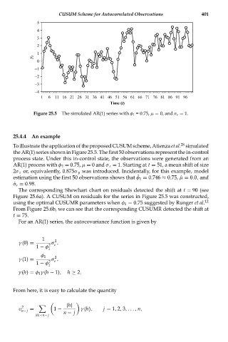
Figure 25.5 The simulated AR(1) series with φ 1 = 0.75, μ = 0, and σ ε = 1.

25.4.4 An example
28
To illustrate the application of the proposed CUSUM scheme, Atienza et al. simulated
the AR(1) series shown in Figure 25.5. The first 50 observations represent the in-control
process state. Under this in-control state, the observations were generated from an
AR(1) process with φ 1 = 0.75, μ = 0 and σ ε = 1. Starting at t = 51, a mean shift of size
2σ ε or, equivalently, 0.875σ y was introduced. Incidentally, for this example, model
estimation using the first 50 observations shows that ˆ φ 1 = 0.746 ≈ 0.75, ˆμ = 0.0, and
ˆ σ ε = 0.98.
The corresponding Shewhart chart on residuals detected the shift at t = 90 (see
Figure 25.6a). A CUSUM on residuals for the series in Figure 25.5 was constructed,
using the optimal CUSUMR parameters when φ 1 = 0.75 suggested by Runger et al. 12
From Figure 25.6b, we can see that the corresponding CUSUMR detected the shift at
t = 75.
For an AR(1) series, the autocovariance function is given by

1 2
γ (0) = 2 σ ,
ε
1 − φ 1
φ 1 2
γ (1) = 2 σ ,
ε
1 − φ 1
γ (h) = φ 1 γ (h − 1), h ≥ 2.

From here, it is easy to calculate the quantity

|h|

υ 2 = 1 − γ (h), j = 1, 2, 3,..., n,
n− j n − j
|h|<n− j