Page 418 - Six Sigma Advanced Tools for Black Belts and Master Black Belts

OTE/SPH
OTE/SPH
Char Count= 0
3:9
August 31, 2006
JWBK119-25
CUSUM Scheme for Autocorrelated Observations 403
Table 25.6 CUSUM mask for an AR(1) process with φ 1 = 0.75, μ = 0, and σ ε = 1 (mw = 10).
n − j γ (n − j) υ 2 Lower arm Upper arm
n− j
9 0.172 10.823 −29.303 29.303
8 0.229 10.362 −27.032 27.032
7 0.305 9.829 −24.628 24.628
6 0.407 9.209 −22.070 22.070
5 0.542 8.484 −19.338 19.338
4 0.723 7.632 −16.405 16.405
3 0.964 5.429 −13.236 13.236
2 1.286 4.000 −9.783 9.783
1 1.714 2.286 −5.938 5.938
0 2.286 0.000 0.000 0.000

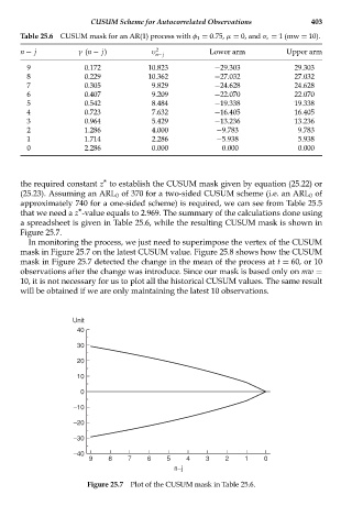
the required constant z * to establish the CUSUM mask given by equation (25.22) or
(25.23). Assuming an ARL 0 of 370 for a two-sided CUSUM scheme (i.e. an ARL 0 of
approximately 740 for a one-sided scheme) is required, we can see from Table 25.5
that we need a z * -value equals to 2.969. The summary of the calculations done using
a spreadsheet is given in Table 25.6, while the resulting CUSUM mask is shown in
Figure 25.7.
In monitoring the process, we just need to superimpose the vertex of the CUSUM
mask in Figure 25.7 on the latest CUSUM value. Figure 25.8 shows how the CUSUM
mask in Figure 25.7 detected the change in the mean of the process at t = 60, or 10
observations after the change was introduce. Since our mask is based only on mw =
10, it is not necessary for us to plot all the historical CUSUM values. The same result
will be obtained if we are only maintaining the latest 10 observations.

Unit
40
30

20
10

0
−10
−20

−30
−40
9 8 7 6 5 4 3 2 1 0
n−j

Figure 25.7 Plot of the CUSUM mask in Table 25.6.