Page 417 - Six Sigma Advanced Tools for Black Belts and Master Black Belts

OTE/SPH
OTE/SPH
3:9
August 31, 2006
Char Count= 0
JWBK119-25
402 CUSUM and Backward CUSUM for Autocorrelated Observations
Residual
4
UCL
3
2
1
0
−1
−2
−3
LCL
−4
0 20 40 60 80 100
(a) Time (t)

CUSUMR
20
15
h = 12.11
10
5
0
−5
−10 h = −12.11
−15
0 20 40 60 80
(b) Time (t)
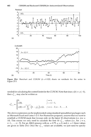
Figure 25.6 Shewhart and CUSUM (k = 0.125) charts on residuals for the series in
Figure 25.5.

needed for calculating the control limits for the CUSUM. Note that since γ (h) = γ (−h),
then υ 2 may also be written as
n− j

⎧
⎪ 0, j = n,
⎪
⎨ γ (0), j = n − 1,
2
υ n− j = n− j−1
⎩γ (0) + 2
1 − i γ (i), j = n − 2, n − 3,..., 1.
⎪
⎪
n− j
i=1
The above expression can be implemented using standard spreadsheet packages such
as Microsoft Excel and Lotus 1-2-3. For illustration purposes, assume that we want to
establish a CUSUM mask that focuses only on the latest 10 observations (i.e. mw =
10). This means we only need to calculate the first 10 υ 2 values (i.e., for j = n,
n− j
n−1,..., n− 9). For an AR(1) process with φ 1 = 0.75, μ = 0, and σ ε = 1 these values
are given in Table 25.6. Once the υ 2 values are available, we just need to specify
n− j