Page 57 - Prosig Catalogue 2005

SOFTWARE PRODUCTS
FATIGUE & DURABILITY TESTING - HOW DO I DO IT?

Training & Support

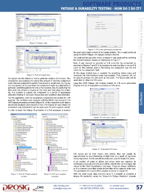
Figure 5: Strain v time

Figure 9: S-N curve generation parameters
the peak and trough content of the captured data. This is easily achieved
using the DATS Fatigue Life Analysis software tool kit.
The peak and trough data shown in Figure 6 was produced by selecting
the relevant analysis module as highlighted in Figure 7.
Next, it was required to generate an S-N curve for the component as
depicted in Figures 7 and 8. It is important to note that this is not an S-N
curve for the material used in fabricating the component, but the S-N Condition Monitoring
curve for the component itself.
At this stage limited data is available for predicting failure rates and
Figure 6: Peak & trough data moreover this information is rough and sporadic. This, however, will not
the signals into the shaker to ‘mimic’ particular sections of the track. This be used to produce the S-N curve at this point. The failure data will be
allowed the test engineers to control the amount of time the component used later to refine the S-N curve.
under test was subjected to specific frequencies or amplitudes. During any Using the DATS Fatigue Life Analysis module for S-N curve generation
one hour period on the test track the component might be subjected to a (Figures 9 & 10) it is possible to produce an S-N curve.
particular excitation pattern for only a few seconds. But, by capturing the
data while the vehicle is moving on the track and then using the shaker
rig, it is possible to subject the component to a period of accelerated
saturation testing of particular frequencies and amplitude characteristics.
For this application note the suspension component was excited for 180
seconds. The excitation was captured with the P8000 and opened in the Software
DATS signal processing software (Figure 5). At this stage the strain data is
stored and displayed with respect to time. The degree of micro strain the
component was subjected to can be seen over the entire capture period.
In order to begin the fatigue life prediction it is first necessary to analyze

Figure 10: S-N curve values

Hardware

Figure 11: Generated S-N curve
S-N curves are by their nature very simple, they can usually be
approximated by two intersecting straight lines on a graph of log stress
verses log cycles. In this case three points are used to create the curve.
A set number of cycles to failure and stress levels are required. As
mentioned previously the S-N curve will be refined later. At this stage, the System Packages
values for the ‘Weld Classification’ are used. These are chosen arbitrarily
as it is a known curve that closely follows that of the material under test.
The generated S-N curve is then created as shown in Figure 11.
Figure 7: Peak & Trough analysis Figure 8: S-N curve analysis With the peak trough data and S-N curve it is possible to complete a
section selection fatigue life prediction, using the ‘Stress Life Fatigue Prediction’ analysis

http://prosig.com +1 248 443 2470 (USA) or contact your 57
sales@prosig.com +44 (0)1329 239925 (UK) local representative
A CMG Company