Page 58 - Prosig Catalogue 2005

SOFTWARE PRODUCTS
FATIGUE & DURABILITY TESTING - HOW DO I DO IT? VIBRATION ANALYSIS: SHOULD WE MEASURE ACCELERATION, VELOCITY OR DISPLACEMENT

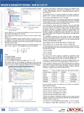
The Fatigue Life Prediction analysis also calculates more detailed results
stored as Named Elements. These are shown highlighted in blue in Figure
15. They include Damage, Duration of original time sample, Number of
cycles and so on.
Training & Support prediction from a sample of strain data taken over a specific time period.
To summarize thus far, it has been possible to complete a fatigue life

This has given a predicted life of 3.4×10 seconds.
20
As discussed earlier, the S-N curve was not a refined curve and was almost
arbitrary in its construction. This could potentially lead to errors. Therefore
at this stage the S-N curve must be refined to allow recalculation of more
accurate results and thus remove any potential errors.

various time periods, hence the reason for the trial. Although the stress
and strain levels are not known for these failures the time to failure
parameters
Figure 12: Stress Life Prediction Figure 13: Stress Life Prediction The component in question has been reported to fail in the field after
is important. Because it is possible to apply the expected strain level
analysis selection for general use to the component for the known period of time, it is,
Condition Monitoring When the analysis module begins it prompts the user for certain values failure is known. 5
therefore, possible to extrapolate the stress levels. Note, the stress levels
module (Figure 12). To complete this analysis both the S-N curve and the
and cycles to failure are not known for these situations. Only the time to
initial peak and trough data are required.
The automotive component was also tested to failure, with failures
(Figure 13).
occurring at the following intervals. As these failures were under controlled
The fatigue life prediction analysis module requires a Young’s modulus for
test environments they can be considered to be more accurate than the
the material, in this case 2.07×10 MPa. A rain flow algorithm must also
5
prediction result discussed previously.
be selected, in this case the ASTM1094. (American Society for Testing and
Time to failure 6.48×10 seconds with a stress of 0.003010 MPa
Materials, Revision 1985).
Time to failure 6.75×10 seconds with a stress of 0.000165 MPa
7
The conversion from Micro Strain to Stress uses the following formula. The
The following have known times to failure, but with unknown strain levels.
, are translated into stress, S, by solving
micro strain values,
For these cases the known failure stress levels can be used, in this case
0.000165 MPa is chosen.
1.52×10 seconds
7
7.78×10 seconds
7
2.64×10 seconds
6
Software E is Young’s Modulus The cycles of the vehicle suspension component, importantly not the
Where
cycles of material, were less that 2Hz. However, the material cycles the
K’ is Strain Hardening Coefficient
component was subjected to were 3253 in a 180 second snap shot.
n’ is Strain Hardening Exponent
If K’ or n’ or both are zero then the module uses
known failure times and then to accurately adjust our initial S-N curve.
This analysis takes two input datasets: the peak and trough count and Therefore, it is possible to calculate the number of material cycles for the
the S-N curve. The resultant ‘Stress Life Fatigue Prediction’ damage curve It is also possible to calculate cycles to failure for the situations where the
is shown in Figure 14, with a fatigue life prediction of 3.4×10 seconds. known failure times do not have strain information. This can be achieved
20
because it is possible from experimental testing to deduce what the
expected or average use and therefore strains will be.
Known or Time to failure Cycles per 180 Cycles to failure
unknown strain (seconds) seconds 11710800
Hardware Known 6.75×10 7 7 3253 1219875000
3253
Known
6.48×10
5
3253
1.52×10
274697777
Unknown
Unknown
2.64×10
Unknown 7.78×10 7 6 3253 1406018888
3253
47710666
Figure 14: Stress Life Prediction data
It is now possible to refine the original S-N curve (Figure 16) with the 5
pairs of values calculated,
0.003010 MPa and 11710800 cycles to failure
System Packages Figure 15: Stress Life Prediction data (Named Elements) 0.000165 MPa and 1406018888 cycles to failure 6
0.000165 MPa and 1219875000 cycles to failure
0.000165 MPa and 274697777 cycles to failure
0.000165 MPa and 47710666 cycles to failure
Therefore it is possible to extrapolate what the S-N curve could have been
and thus re-process the results using the automatic reprocessing features
of DATS as shown in Figure 16.
The result of the re-processed fatigue life prediction is 4.40×10 seconds.
The conclusion is that after approximately 51 days of use at the
58 http://prosig.com +1 248 443 2470 (USA) or contact your
+44 (0)1329 239925 (UK) local representative
sales@prosig.com
A CMG Company