Page 276 - Maxwell House

256 ANTENNA BASICS

literature [16]. Suppose that the desired communication channel bandwidth is ∆ = 1 THz =
10 Hz whereas the optic frequencies are around = 10 Hz. Therefore, the photonic channel,
14
9
carrying this ultra-broadband signal consumes the relative bandpass ∆ = 10 or 0.001%.
−5
⁄
We can certainly forget about any detectable dispersion in such an extremely narrow-banded
channel. Note that according to the Shannon theorem, the capacity of this channel in bit rate is
= ∆ log (1 + ) = 10 log (1 + 10) = 2.4 ∙ 10 bits/s or 61 Terabytes/s with
9
9
2 2
moderate SNR = 10. You would be able to download around a million Ultra HD TV channels
per second!
Meanwhile, the trend of shifting the broadband signal generation, transmission, and processing
to an optical frequency band is quickly gaining momentum. The main benefits of
optoelectronics is the decrease in cost, size and weight, low noise figures and high dynamic
range over a wide RF bandwidth, immunity to EM and RF interference, high reliability and
security against signal interception, “install and forget” maintenance technology, etc.

5.5.5 Frequency Scan

Finally, it is worth noting that beam squint is not always a negative effect. In fact, some of the
earliest phased arrays used this property to steer the beam in what are called frequency-scan
arrays. Let us come back to Figure
5.4.9b and replace the fixed phase
shifters with dispersive transmission
line sections of equal length ∆ as
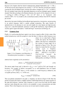
depicted in Figure 5.5.6a. The term
dispersive means that the wave phase
velocity () is frequency

dependent while the inter-element
phase shift () = − ()∆ =
Figure 5.5.6 a) Frequency scan illustration, b) (2 () ∆ becomes the

Normalized polar scan pattern vs. frequency ⁄
nonlinear function of frequency.
Subsequently, according to (5.89) the
antenna factor magnitude can be presented as

⁄
sin ((+1)(cos−(∆ ()))/2)
() = 0 (5.95)
sin ((cos−(∆ ()))/2)
⁄
−1 (∆ ()) and depends on,
The pattern main beam peak is directed to = cos ⁄
frequency. For example, in hollow waveguides, as we will demonstrate later in Chapter
6, () = �1 − ( )⁄ ⁄ 2 where is the constant (i.e. cutoff frequency) defined by the

waveguide geometry and > . In this case,

2
⁄
= cos(∆�1 − ( ) � ) (5.96)

The scan patterns normalized to the peak vs. frequency are shown in Figure 5.5.6b. Here the
picture-in-picture plot depicts a slightly nonlinear relationship between the angular position of
the peak and frequency variation. Since frequency is used to steer the beam, the RF signal
spectrum varies during the scan, which is not acceptable in many communication and radar
systems. This is why frequency-scan arrays are not used much in modern systems.