Page 298 - Maxwell House

278 Chapter 6

E-field distribution over transverse coordinates can be found from (6.2) as the solution of
Laplace’s equation while the magnetic field is defined by (6.3)
2
∇ (, ) = 0
0 � (6.5)
(, ) = � × (, )
0
0
The “chasing us” again and again is the parameter of the free space impedance =
0
|(, )| |(, )| = � = 376.73� ≅ 120� [Ω] is the ratio of the
⁄
⁄
⁄
⁄

0
0

transverse component of the electric and magnetic fields in line. Note that in the literature this
impedance is denoted sometimes by symbol . The remarkable fact is the frequency completely
disappeared from equations in (6.5). Therefore, if the solution of (6.5) occurs it must be
frequency independent and, in particular, has to be the same as static (DC) at = 0.
Nevertheless, DC power line requires as minimum two separated conductive wires to deliver
power to the load: one wire is the forward path for the electrical current while a second and
separated one is needed as the current return path. From this fact follows that the EM wave
(6.5) can really propagate and carry energy in any line if and only if it is capable to deliver DC
power. Evidently, all lines demonstrated later in Figure 6.2.1a and b (except one-wire Goubau’s
line) meet this requirement.
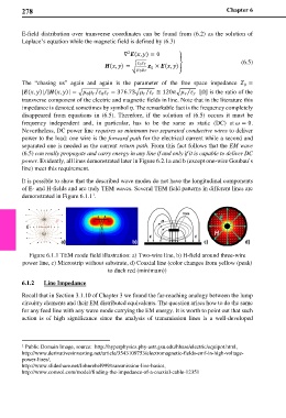
It is possible to show that the described wave modes do not have the longitudinal components
of E- and H-fields and are truly TEM waves. Several TEM field patterns in different lines are
demonstrated in Figure 6.1.1 .
1

Figure 6.1.1 TEM mode field illustration: a) Two-wire line, b) H-field around three-wire
power line, c) Microstrip without substrate, d) Coaxial line (color changes from yellow (peak)
to duck red (minimum))

6.1.2 Line Impedance

Recall that in Section 3.1.10 of Chapter 3 we found the far-reaching analogy between the lump
circuitry elements and their EM distributed equivalents. The question arises how to do the same
for any feed line with any wave mode carrying the EM energy. It is worth to point out that such
action is of high significance since the analysis of transmission lines is a well-developed

1 Public Domain Image, source: http://hyperphysics.phy-astr.gsu.edu/hbase/electric/equipot.html,
http://www.derivativesinvesting.net/article/3543109753/electromagnetic-fields-emf-in-high-voltage-
power-lines/,
http://www.slideshare.net/Johnrebel999/transmission-line-basics,
http://www.comsol.com/model/finding-the-impedance-of-a-coaxial-cable-12351