Page 299 - Maxwell House

FEED LINE BASICS 279

analytically and numerically section of classical circuit theory. The logical connection is based
as usual on the fundamental physical principle of energy conservation.
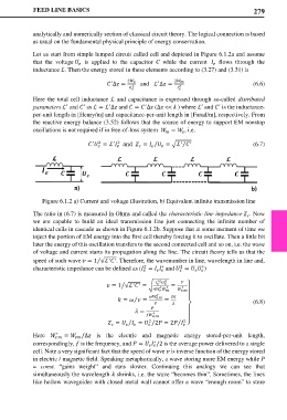
Let us start from simple lumped circuit called cell and depicted in Figure 6.1.2a and assume
that the voltage is applied to the capacitor C while the current flows through the

inductance ℒ. Then the energy stored in these elements according to (3.27) and (3.31) is
′
′
∆ = 2 and ℒ ∆ = 2 (6.6)
2 2

Here the total cell inductance ℒ and capacitance is expressed through so-called distributed
parameters ℒ and as ℒ = ℒ ∆ and = ∆ (∆ << ) where ℒ and is the inductance-
′
′
′
′
′
′
per-unit length in [Henry/m] and capacitance-per-unit length in [Farad/m], respectively. From
the reactive energy balance (3.52) follows that the source of energy to support EM nonstop
oscillations is not required if in free-of-loss system = , i.e.

= ℒ and = = �ℒ (6.7)
2
′
′ 2
′
′
⁄
⁄

Figure 6.1.2 a) Current and voltage illustration, b) Equivalent infinite transmission line
The ratio in (6.7) is measured in Ohms and called the characteristic line impedance . Now

we are capable to build an ideal transmission line just connecting the infinite number of
identical cells in cascade as shown in Figure 6.1.2b. Suppose that at some moment of time we
inject the portion of EM energy into the first cell thereby forcing it to oscillate. Then a little bit
later the energy of this oscillation transfers to the second connected cell and so on, i.e. the wave
of voltage and current starts its propagation along the line. The circuit theory tells us that the
speed of such wave = 1 √ℒ . Therefore, the wavenumber in line, wavelength in line and,
′
′
⁄
characteristic impedance can be defined as ( = and = )
2
2
∗
∗

∗2 2

= 1 √ℒ = �� ′ ′ = ⎫
′ ′ ′
4 ,
⎪
′ ⎪
, 2
⁄
= = = (6.8)

⎬
=
′ ⎪
, ⎪
= = ⁄⁄ 2 2 = 2 ⁄ 2 ⎭

′
Here , = /∆ is the electric and magnetic energy stored-per-unit length,

correspondingly, is the frequency, and = /2 is the average power delivered to a single
∗

cell. Note a very significant fact that the speed of wave is inverse function of the energy stored
in electric / magnetic field. Speaking metaphorically, a wave storing more EM energy while P
= const. “gains weight” and runs slower. Continuing this analogy we can see that
simultaneously the wavelength shrinks, i.e. the wave “becomes thin”. Sometimes, the lines
like hollow waveguides with closed metal wall cannot offer a wave “enough room” to store