Page 177 - Mechatronics with Experiments

MECHANISMS FOR MOTION TRANSMISSION 163

T
04
T
23 θ 3 T 34
y
3
y z
2 y
4 4
x x
2 3
T 12 θ
θ z 3 4
2
x
4
z
2 x
1 r
θ 4A
1
y z
1 1
T z 0 r OA
01 A
y
0
x
0
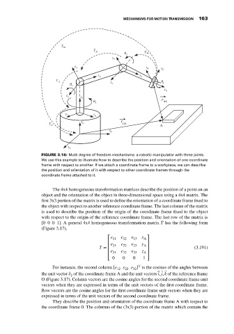
FIGURE 3.16: Multi degree of freedom mechanisms: a robotic manipulator with three joints.
We use this example to illustrate how to describe the position and orientation of one coordinate
frame with respect to another. If we attach a coordinate frame to a workpiece, we can describe
the position and orientation of it with respect to other coordinate frames through the
coordinate frame attached to it.

The 4x4 homogeneous transformation matrices describe the position of a point on an
object and the orientation of the object in three-dimensional space using a 4x4 matrix. The
first 3x3 portion of the matrix is used to define the orientation of a coordinate frame fixed to
the object with respect to another reference coordinate frame. The last column of the matrix
is used to describe the position of the origin of the coordinate frame fixed to the object
with respect to the origin of the reference coordinate frame. The last row of the matrix is
[0001]. A general 4x4 homogeneous transformation matrix T has the following form
(Figure 3.17),

⎡ e 11 e 12 e 13 x ⎤
A
e 21 e 22 e 23 y A
⎢ ⎥
T = ⎢ ⎥ (3.191)
⎢ e e e
31 32 33 z ⎥
A
⎢ ⎥
⎣ 0 0 0 1 ⎦
T
For instance, the second column [e e e ] is the cosines of the angles between
12 22 32
⃗
the unit vector ⃗ e of the coordinate frame A and the unit vectors ⃗ i, ⃗ j, k of the reference frame
2
O (Figure 3.17). Column vectors are the cosine angles for the second coordinate frame unit
vectors when they are expressed in terms of the unit vectors of the first coordinate frame.
Row vectors are the cosine angles for the first coordinate frame unit vectors when they are
expressed in terms of the unit vectors of the second coordinate frame.
They describe the position and orientation of the coordinate frame A with respect to
the coordinate frame 0. The columns of the (3x3) portion of the matrix which contain the