Page 83 - Mechatronics with Experiments

CLOSED LOOP CONTROL 69
Therefore, if it is desired that the closed loop system (CLS) step response should not have
more than a certain amount of PO%, and should settle down within ±2% of the final value
within t (seconds), the designer must seek a controller which will make the closed loop
s
system behave like (or similar to) a second-order system whose two poles are given by the
above relationships.

2.5 TIME DOMAIN AND S-DOMAIN
CORRELATION OF SIGNALS

The response of a linear time invariant dynamic system, y(t), as a result of an input signal,
r(t) can be calculated using the Laplace transforms

y(s) = G(s) r(s)

The impulse response y(s) can be expanded to its partial fraction expansion (PFE) which
has the general form as follows,
m m
1 ∑ A i ∑ B j
y(s) = + + ( )
2
s s + i s + 2 s + + 2
2
i=1 j=1 j j i
A , B − residue of PFE of G(s) r(s)
i
j
The time domain response, y(t) can be obtained by taking the inverse Laplace transform of
each term of the PFE,
m m ( )
∑ − i t ∑ − j t 1
y(t) = 1(t) + A e + B e sin t
i j j
i=1 j=1 j
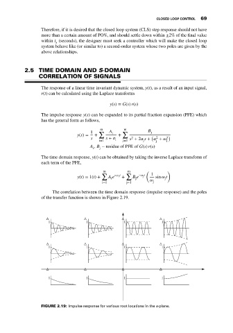
The correlation between the time domain response (impulse response) and the poles
of the transfer function is shown in Figure 2.19.

1 1 1 1

1 1 1 1

1 1 1 1

FIGURE 2.19: Impulse response for various root locations in the s-plane.