Page 88 - Mechatronics with Experiments

74 MECHATRONICS

ω 2
s ω B 2 + 2ξ ω s ω B + ω 2 Same

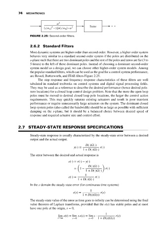
FIGURE 2.25: Second-order filters.

2.6.2 Standard Filters

Most dynamic systems are higher order than second order. However, a higher order system
behaves very similar to a standard second-order system if the poles are distributed on the
s-plane such that there are two dominant poles and the rest of the poles and zeros are far (3 to
5 times) to the left of these dominant poles. Instead of choosing a dominant second-order
system model as a design goal, we can choose other higher-order system models. Among
the popular standard filters, which can be used as the goal for a control system performance,
are Bessel, Butterworth, and ITAE filters Figure 2.25.
The step response and frequency response characteristics of these filters are well
tabulated in standard textbooks on control systems and digital signal processing fields.
They may be used as a reference to describe the desired performance (hence desired pole-
zero locations) for a closed loop control design problem. Note that the more the open loop
poles must be moved to desired closed loop pole locations, the larger the control action
requirements. This may quickly saturate existing actuators and result in poor transient
performance or require unnecessarily large actuators on the system. The dominant closed
loop system poles (also called the bandwidth) should be as large as possible with sufficient
damping on the s-plane, but it should be a balanced choice between desired speed of
response and required actuator size and control effort.

2.7 STEADY-STATE RESPONSE SPECIFICATIONS

Steady-state response is usually characterized by the steady-state error between a desired
output and the actual output.
D(⋅)G(⋅)
y(⋅) = r(⋅)
1 + D(⋅)G(⋅)
The error between the desired and actual response is
e(⋅) = r(⋅) − y(⋅)
( )
D(⋅)G(⋅)
= 1 − r(⋅)
1 + D(⋅)G(⋅)
1
e(⋅) = r(⋅)
1 + D(⋅)G(⋅)
In the s-domain the steady-state error (for continuous time systems)
1
e(s) = r(s)
1 + D(s)G(s)
The steady-state value of the error as time goes to infinity can be determined using the final
value theorem of Laplace transforms, provided that the e(s) has stable poles and at most
have one pole at the origin, s = 0,
1
lim e(t) = lim se(s) = lim s ⋅ r(s)
t→∞ s→0 s→0 1 + D(s)G(s)