Page 208 - Servo Motors and Industrial Control Theory -

Appendix B 205

−Ts
where the transfer function of a transport lag is ( e ). This transfer function
cannot be dealt with easily. Without going into detail of the proof such transfer
function can be approximated by,
Ts (Ts) 2 (Ts) 3
1 − + − +
2
8
48
e − Ts = : Ts (Ts) 2 (Ts) 3
1 + + − +
2 8 48
Depending on the system and the accuracy required for analysis of the system
a number of terms both the numerator and denominator of the above equation
can be selected. You should remember that the transport lag becomes signifi-
cant when the dead time is in the range of system response time.
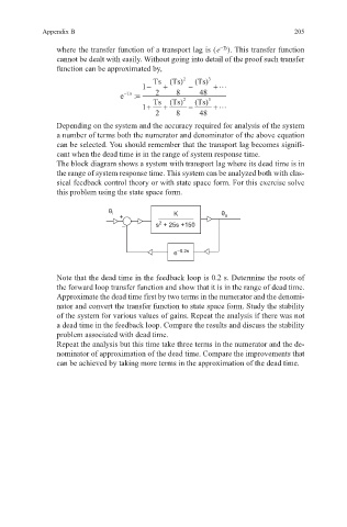
The block diagram shows a system with transport lag where its dead time is in
the range of system response time. This system can be analyzed both with clas-
sical feedback control theory or with state space form. For this exercise solve
this problem using the state space form.

θ i K θ
+ o
2
– s + 25s +150

e –0.2s

Note that the dead time in the feedback loop is 0.2 s. Determine the roots of
the forward loop transfer function and show that it is in the range of dead time.
Approximate the dead time first by two terms in the numerator and the denomi-
nator and convert the transfer function to state space form. Study the stability
of the system for various values of gains. Repeat the analysis if there was not
a dead time in the feedback loop. Compare the results and discuss the stability
problem associated with dead time.
Repeat the analysis but this time take three terms in the numerator and the de-
nominator of approximation of the dead time. Compare the improvements that
can be achieved by taking more terms in the approximation of the dead time.