Page 184 - Theoretical and Practical Interpretation of Investment Attractiveness

against real data. Among them, the most discussed in the econometric literature are
endogeneity problems. According to the Gauss-Markov theorem, among fixed estimators,
parameters estimated by the EKK method have the smallest standard error or variance, but
each of the above conditions is often violated in real situations.
In particular, ܧሺݑȁܺሻ ൌܧሺݑȁݔ ǡݔ ǡǥǡݔ ሻ ൌͲas a result of the action of exogenous
ଵ ଶ ௞
regressors, i.e., violation of the hypothesis, the parameters calculated using the EKC method
deviate from the real ones, and decisions made using the calculated parameters can lead to
incorrect and unexpected results.
Although there are several reasons for the endogeneity problem, the most important is
the variables excluded from the regression model. The more these variables influence the
independent variable, the more serious the endogeneity problem. Of course, adding omitted
variables to the regression model solves the problem, but often information about the omitted
variables is not available.
For example, in this study, although the culture and customs of investors are one of the
necessary factors influencing the amount of investment, this variable amount is difficult to
measure and statistics on it are not collected.
As a second example, Uzbekistan's mineral reserves are of interest to investors, but
since this area is of strategic importance, information is difficult to obtain. Therefore, although
these factors influence investor behavior, there is no choice but to ignore it, and therefore the
problem of endogeneity remains.
Panel data, unlike cross-sectional samples and time series, reduce the problem of
endogeneity by controlling for unobserved heterogeneity, that is, unobserved differences
between panel units, especially between panel units that do not change over time. It is for this
reason that panel models are tested as the econometric models used in this study.
Taking into account the peculiarities of working with panel data, below we will touch
on some of their important aspects.
A conditional definition of indicators used to carry out planned actions is required.
࢟ - the value of an arbitrary variable corresponding to time t for the i-panel block,
࢏࢚
where ݅ ൌ ͳǡǥ ǡ ܰǡݐ ൌ ͳǡǥ ǡܶ;
࢐
࢞ - value of the independent variable corresponding to time t for the i-panel block
࢏࢚
௝
ݔ ; Here ݆ൌ ͳǡǥ ǡ ݇.
In our model ܰൌ ͳͶ ൐ ͳandʡൌ ͳ͹ ൐ ͳ ham_ _ܰ൏ ܶ hence the panel in question
is a "long" panel . Here N is the number of observed panel units, and T is the observation
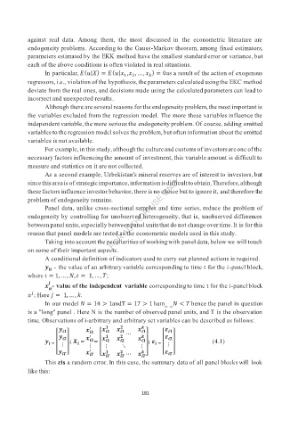
time. Observations of i-arbitrary and arbitrary set variables can be described as follows:
࢟ ࢏૚ ࢞ ᇱ ࢏૚ ۍ ࢞ ૚ ࢏૚ ࢞ ૛ ࢏૚ ࢞ ࢑ ࢏૚ ې ࢿ ࢏૚
࢟ ࢏૛ ࢞ ᇱ ࢏૛ ێ ࢞ ૚ ࢞ ૛ ڮ ࢞ ࢑ ࢿ ࢏૛
࢟ ࢏ ୀ ൦ ڭ ൪; ࢄ = ڭ = ێ ڭ ࢏૚ ࢏૛ ڰ ڭ ࢏૚ۑ ۑ ; ࢿ ࢏ ୀ ൦ ڭ ൪ (4.1)
࢏
࢟ ࢏ࢀ ࢞ ᇱ ࢏ࢀ ۏ࢞ ૚ ࢏ࢀ ࢞ ڮ ૛ ࢏ࢀ ࢞ ࢑ ࢏ࢀ ے ࢿ ࢏ࢀ
This ࢿis a random error. In this case, the summary data of all panel blocks will look
like this:

181