Page 185 - Theoretical and Practical Interpretation of Investment Attractiveness

࢟ ૚ ࢄ ૚ ࢿ ૚
࢟ ૛ ࢄ ࢿ ૛
࢟ ࢏ ୀ ൦ ڭ ൪; ࢄ "= ڭ ૛ " ࢿ ࢏ ୀ ൦ ڭ ൪; (4.2)
࢏
࢟ ࡺ ࢄ ࡺ ࢿ ࡺ
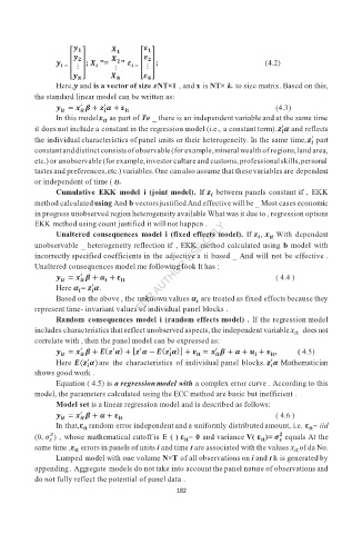
Here,࢟ and is a vector of size ࢿNT×1 , and x is NT× k. to size matrix. Based on this,
the standard linear model can be written as:
ᇱ ᇱ
࢟ ൌ࢞ ࢼ൅ ࢠ ࢻ൅ ઽ (4.3)
ܑܜ
࢏࢚
࢏
࢏࢚
In this model࢞ as part of To _ there is an independent variable and at the same time
࢏࢚
ᇱ
it does not include a constant in the regression model (i.e., a constant term).ࢠ ࢻ and reflects
࢏
ᇱ
the individual characteristics of panel units or their heterogeneity. In the same time,ࢠ part
࢏
constant and distinct consists of observable (for example, mineral wealth of regions, land area,
etc.) or unobservable (for example, investor culture and customs, professional skills, personal
tastes and preferences, etc.) variables. One can also assume that these variables are dependent
or independent of time ( t).
Cumulative EKK model i (joint model). If ࢠ between panels constant if , EKK
࢏
method calculated using And b vectors justified And effective will be _ Most cases economic
in progress unobserved region heterogeneity available What was it due to , regression options
EKK method using count justified it will not happen .
Unaltered consequences model i (fixed effects model). If ࢠ , ࢞ With dependent
࢏
࢏࢚
unobservable _ heterogeneity reflection if , EKK method calculated using b model with
incorrectly specified coefficients in the adjective a ti based _ And will not be effective .
Unaltered consequences model me following look It has :
ᇱ
࢟ ൌ࢞ ࢼ൅ ࢻ ൅ઽ ( 4.4 )
࢏࢚
࢏࢚
࢏
ܑܜ
ᇱ
Here ࢻ = ࢠ ࢻ.
࢏
࢏
Based on the above , the unknown values ࢻ are treated as fixed effects because they
࢏
represent time- invariant values of individual panel blocks .
Random consequences model i (random effects model) . If the regression model
includes characteristics that reflect unobserved aspects, the independent variableݔ does not
௜௧
correlate with , then the panel model can be expressed as:
ᇱ ᇱ ᇱ ᇱ ᇱ
࢟ ൌ࢞ ࢼ൅ ࡱሺࢠ ࢻሻ ൅ ༰ࢠ ࢻെ ࡱሺࢠ ࢻሻ༱ ൅ઽ ൌ࢞ ࢼ൅ ࢻ ൅ ࢛ ൅ઽ , ( 4.5)
ܑܜ
ܑܜ
࢏࢚
࢏࢚
࢏
࢏࢚
࢏
ᇱ
ᇱ
Here ࡱሺࢠ ࢻሻare the characteristics of individual panel blocks. ࢠ ࢻ Mathematician
࢏
࢏
shows good work .
Equation ( 4.5) is a regression model with a complex error curve . According to this
model, the parameters calculated using the ECC method are basic but inefficient .
Model set is a linear regression model and is described as follows:
ᇱ
࢟ ൌ࢞ ࢼ൅ ࢻ ൅ ઽ ( 4.6 )
࢏࢚
࢏࢚
ܑܜ
In that,ઽ random error independent and a uniformly distributed amount, i.e. ઽ ~ iid
ܑܜ
ܑܜ
ଶ
૛
(0, ߪ ) , whose mathematical cutoff is E ( ) ઽ = 0 and variance V( ઽ )= ࣌ equals At the
ఌ ܑܜ ܑܜ ࢿ
same time ,ઽ errors in panels of units i and time t are associated with the values ݔ of da No.
௜௧
ܑܜ
Lumped model with one volume N×T of all observations on i and t h is generated by
appending . Aggregate models do not take into account the panel nature of observations and
do not fully reflect the potential of panel data .
182