Page 190 - Theoretical and Practical Interpretation of Investment Attractiveness

෢
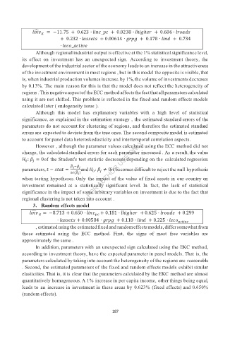
݈ଓ݊ݒ ൌ െͳͳǤ͹ͷ ൅ ͲǤ͸ʹ͵ ή ̴݈݅݊ܿ݌ܿ ൅ ͲǤͲʹ͵ͺ ή ݈݄݄݅݃݁ݎ ൅ ͲǤ͸ͺ͸ ή ݈ݎ݋ܽ݀ݏ
௜௧
൅ ͲǤʹ͵ʹ ή ݈ܽݏݏ݁ݐݏ ൅ ͲǤͲͲ͸ͳͶ ή ݃ݎ݌݃ ൅ ͲǤͳ͹ͺ ή ݈݅݊݀ ൅ ͲǤ͹͵Ͷ
ή݈݁ܿ݋̴ܽܿݐ݅ݒ݁
Although regional industrial output is effective at the 1% statistical significance level,
its effect on investment has an unexpected sign. According to investment theory, the
development of the industrial sector of the economy leads to an increase in the attractiveness
of the investment environment in most regions , but in this model the opposite is visible, that
is, when industrial production volumes increase. by 1%, the volume of investments decreases
by 0.13%. The main reason for this is that the model does not reflect the heterogeneity of
regions . This negative aspect of the ECC method affects the fact that all parameters calculated
using it are not shifted. This problem is reflected in the fixed and random effects models
calculated later ( endogeneity issue ).
Although this model has explanatory variables with a high level of statistical
significance, as explained in the estimation strategy , the estimated standard errors of the
parameters do not account for clustering of regions, and therefore the estimated standard
errors are expected to deviate from the true ones. The second composite model is estimated
to account for panel data heteroskedasticity and intertemporal correlation aspects.
However , although the parameter values calculated using the ECC method did not
change, the calculated standard errors for each parameter increased . As a result, the value
ܪ ǣ ߚ ൌͲof the Student's test statistic decreases depending on the calculated regression
଴
௝
ೕ
ఉ ෡ ିఉ ೕ
parameters, ݐെݏݐܽݐ ൌ and ܪ ǣ ߚ ്Ͳit becomes difficult to reject the null hypothesis
଴
௝
௦௘ሺఉ ෡ ሻ
ೕ
when testing hypotheses. Only the impact of the value of fixed assets in our country on
investment remained at a statistically significant level. In fact, the lack of statistical
significance in the impact of some arbitrary variables on investment is due to the fact that
regional clustering is not taken into account .
3. Random effects model
෢
݈ଓ݊ݒ ൌ െͺǤ͹ͳ͵ ൅ ͲǤ͸ͷͲ ή ݈݅݊ܿ ௣௖ ൅ ͲǤͳͺͳ ή ݈݄݄݅݃݁ݎ ൅ ͲǤ͸ʹͷ ή ݈ݎ݋ܽ݀ݏ ൅ ͲǤʹͻͻ
௜௧
ή ݈ܽݏݏ݁ݐݏ ൅ ͲǤͲͲͷͺͶ ή ݃ݎ݌݃ ൅ ͲǤͳͳͺ ή ݈݅݊݀ ൅ ͲǤʹʹͷ ή ݈݁ܿ݋ ௔௖௧௜௩௘
, estimated using the estimated fixed and random effects models, differ somewhat from
those estimated using the ECC method. First, the signs of most free variables are
approximately the same .
In addition, parameters with an unexpected sign calculated using the EKC method,
according to investment theory, have the expected parameter in panel models. That is, the
parameters calculated by taking into account the heterogeneity of the regions are reasonable
. Second, the estimated parameters of the fixed and random effects models exhibit similar
elasticities. That is, it is clear that the parameters calculated by the EKC method are almost
quantitatively homogeneous. A 1% increase in per capita income, other things being equal,
leads to an increase in investment in these areas by 0.623% (fixed effects) and 0.650%
(random effects).

187