Page 606 - NGTU_paper_withoutVideo

Modern Geomatics Technologies and Applications

(GI) is used for CART implementation in R as the splitting criterion. It measures the degree of a particular
randomly chosen item of a data being wrongly classified, calculated in (1) [15]:

2
= 1 − ∑ , (1)

=1

where is the relative frequency of class in the dataset. During the training process, an optimal value for

Complexity Parameter (CP) is determined. This time-saver parameter prunes off the unimportant splits. In other
words, any split which does not improve the fit by CP will be pruned off by cross validation.

4.1.2. C5.0 tree: C5.0 is an improved version of C4.5 tree, which is also an extension of ID3 algorithm developed by
Quinlan [16]. The algorithm uses information gain as the splitting criterion and gives a binary or multi branches
tree. In comparison with C4.5, C5.0 accounts for missing values, dates, times and ordered variables. Moreover,
it has a faster functionality, less memory consumption. The tree structure uses boosting, i.e. many generated
decision trees are combined together to improve the prediction. A variable with the highest information gain is
chosen as the splitting variable of the root node. Then the algorithm is recursively applied to each branch to build
the nodes and branches. In order to define information gain, the entropy must be introduced first. entropy is an
impurity measure in the dataset, defined as (2) [17]:

| |
( ) = − ∑ log , (2)

2

=1

where refers to the train data and is the probability that an item in the train data belongs to class . If the

data consists of just one class, then would be 1 and the entropy would be zero. Therefore, the entropy for a

homogeneous dataset would be minimized. As mentioned before, an optimal variable is needed to split the tree
node to minimize the tree depth, implying that the variable with the most entropy reduction is the ideal choice.
Given by equation (3), the information gain for each variable can be defined as the difference between the
entropies of the dataset and the weighted sum of the entropies from the data subsets [17]:

| |

( , ) = ( ) − ∑ × ( ), (3)
| |
=1

Where | |is the number of train data, is a variable in the dataset with different values, is the samples in
every value, and | | is the number of these samples. Three parameters are optimized after the training process:

1. The number of boosting iterations, called trials. 2. A logical value whether to decompose the tree into a rule-
based model or not, denoted as model. 3. Another logical value whether to use feature selection or not, denoted
as winnow.

4.2. Classification Evaluation Metrics

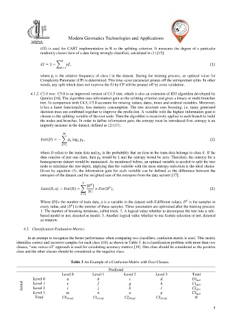
In an attempt to recognize the better performance when comparing two classifiers, confusion matrix is used. This matrix
identifies correct and incorrect samples for each class [18], as shown in Table 3. In a classification problem with more than two
classes, “one versus all” approach is used for calculating accuracy metrics [19]. One class should be considered as the positive
class and the other classes should be considered as the negative class.

Table 3 An Example of a Confusion Matrix with Four Classes.

Predicted
Level 0 Level 1 Level 2 Level 3 Total
Level 0 0
Actual Level 1 ℎ 1
Level 2

2
Level 3 3

Total 0 1 2 3

4