Page 102 - u4

P2: OSO/OVY
QC: OSO/OVY
T1: OSO
P1: OSO/OVY
13:38
July 4, 2016
GO01962-Smith-v1.cls
UAE_Math_Grade_12_Vol_1_SE_718383_ch3
of the object of a given volume is the same), then the mass density is simply
mass density = mass
volume
and this quantity is constant throughout the object. However, if the mass of a given
volume varies in different parts of the object, then this formula only calculates the
average density of the object. In example 9.6 we find a means of computing the mass
density at a specific point in a nonhomogeneous object.
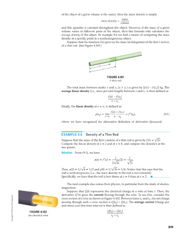
Suppose that the function f(x) gives us the mass (in kilograms) of the first x meters
of a thin rod. (See Figure 4.101.)

x 1
x

FIGURE 4.101
A thin rod

The total mass between marks x and x (x > x ) is given by [f(x) − f(x )] kg. The
1
1
1
average linear density (i.e., mass per unit length) between x and x is then defined as
1
f(x) − f(x )
1
x − x 1 .
Finally, the linear density at x = x is defined as
1
f(x) − f(x )
′
(x ) = lim 1 = f (x ), (9.1)
1
1
x→x 1 x − x 1
where we have recognized the alternative definition of derivative discussed.
EXAMPLE 9.6 Density of a Thin Rod
√
Suppose that the mass of the first x meters of a thin rod is given by f(x) = 2x.
Compute the linear density at x = 2 and at x = 8, and compare the densities at the
two points.
Solution From (9.1), we have
′ 1 1
(x) = f (x) = √ (2) = √ .
2 2x 2x
√ √
Thus, (2) = 1∕ 4 = 1∕2 and (8) = 1∕ 16 = 1∕4. Notice that this says that the
rod is nonhomogeneous (i.e., the mass density in the rod is not constant).
Specifically, we have that the rod is less dense at x = 8 than at x = 2.

The next example also comes from physics, in particular from the study of electro-
magnetism.
Suppose that Q(t) represents the electrical charge in a wire at time t. Then, the
′
derivative Q (t) gives the current flowing through the wire. To see this, consider the
Copyright © McGraw-Hill Education An electrical wire passing through such a cross section is Q(t ) − Q(t ). The average current (charge per
cross section of a wire as shown in Figure 4.102. Between times t and t , the net charge
1
2
1
2
unit time) over this time interval is then defined as
Q(t ) − Q(t )
FIGURE 4.102
2
1
.
t − t
1
2
311