Page 103 - u4

QC: OSO/OVY
T1: OSO
P2: OSO/OVY
P1: OSO/OVY
UAE_Math_Grade_12_Vol_1_SE_718383_ch3
GO01962-Smith-v1.cls
13:38
July 4, 2016
The instantaneous current I(t) at any time t can then be found by computing the limit
1
Q(t) − Q(t )
′
I(t ) = lim 1 = Q (t ), (9.2)
1
1
t→t 1 t − t 1
since (9.2) is again the alternative definition of derivative.
14 ohms 0.05 farad
EXAMPLE 9.7 Modeling Electrical Current in a Wire
The electrical circuit shown in Figure 4.103 includes a 14-ohm resistor, a 2-henry
2 henrys inductor, a 0.05-farad capacitor and a battery supplying 232 volts of AC current
modeled by the oscillating function 232 sin 2t, where t is measured in seconds. Find
~ the current in the circuit at any time t.
232 volts Solution It can be shown (using the elementary laws of electricity) that the charge
in this circuit is given by
FIGURE 4.103
A simple electrical circuit Q(t) = 10e −5t + 2te −2t + 3 sin 2t − 7 cos 2t coulombs.

The current is then
p
′
Q (t) =−50e −5t + 2e −2t − 4te −2t + 6 cos 2t + 14 sin 2t amps (coulombs per second).
1

0.8 We have briefly explored the rate of growth of a population. Population
dynamics is an area of biology that makes extensive use of calculus. For now, we
0.6 explore one aspect of a basic model of population growth called the logistic equation.
This states that if p(t) represents population (measured as a fraction of the maximum
0.4
sustainable population), then the rate of change of the population satisfies the
equation
0.2
′
t p (t) = rp(t)[1 − p(t)],
2 4 6 8
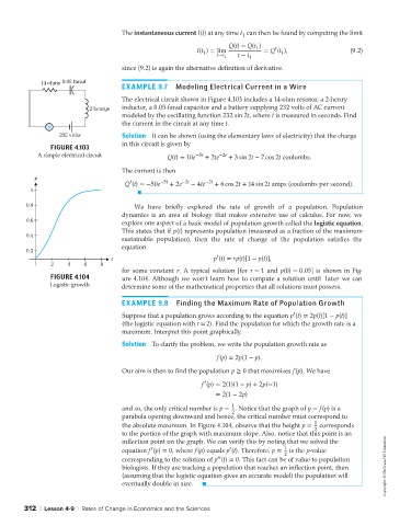
for some constant r. A typical solution [for r = 1 and p(0) = 0.05] is shown in Fig-
FIGURE 4.104 ure 4.104. Although we won’t learn how to compute a solution until later we can
Logistic growth determine some of the mathematical properties that all solutions must possess.

EXAMPLE 9.8 Finding the Maximum Rate of Population Growth
′
Suppose that a population grows according to the equation p (t) = 2p(t)[1 − p(t)]
(the logistic equation with r = 2). Find the population for which the growth rate is a
maximum. Interpret this point graphically.
Solution To clarify the problem, we write the population growth rate as

f(p) = 2p(1 − p).
Our aim is then to find the population p ≥ 0 that maximizes f(p). We have
′
f (p) = 2(1)(1 − p) + 2p(−1)
= 2(1 − 2p)
1
and so, the only critical number is p = . Notice that the graph of y = f(p)isa
2
parabola opening downward and hence, the critical number must correspond to
the absolute maximum. In Figure 4.104, observe that the height p = 1 corresponds
2
to the portion of the graph with maximum slope. Also, notice that this point is an
inflection point on the graph. We can verify this by noting that we solved the
′
′
equation f (p) = 0, where f(p) equals p (t). Therefore, p = 1 2 is the p-value
′′
corresponding to the solution of p (t) = 0. This fact can be of value to population
biologists. If they are tracking a population that reaches an inflection point, then Copyright © McGraw-Hill Education
(assuming that the logistic equation gives an accurate model) the population will
eventually double in size.

312 | Lesson 4-9 | Rates of Change in Economics and the Sciences