Page 99 - u4

P2: OSO/OVY
P1: OSO/OVY
GO01962-Smith-v1.cls
UAE_Math_Grade_12_Vol_1_SE_718383_ch3
To minimize C(x), we start by finding critical numbers in the domain x > 0. We have
y QC: OSO/OVY T1: OSO July 4, 2016 13:38
30 ′
C (x) = 0.02 − 4000x −2 = 0 if
25
4000x −2 = 0.02 or
20
4000 2
15 0.02 = x .
10 √
2
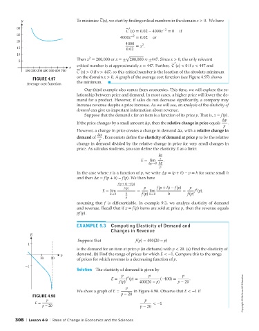
Then x = 200,000 or x =± 200,000 ≈±447. Since x > 0, the only relevant
5 ′
critical number is at approximately x = 447. Further, C (x) < 0 if x < 447 and
x ′
100 200 300 400 500 600 700 C (x) > 0 if x > 447, so this critical number is the location of the absolute minimum
on the domain x > 0. A graph of the average cost function (see Figure 4.97) shows
FIGURE 4.97
Average cost function the minimum.
Our third example also comes from economics. This time, we will explore the re-
lationship between price and demand. In most cases, a higher price will lower the de-
mand for a product. However, if sales do not decrease significantly, a company may
increase revenue despite a price increase. As we will see, an analysis of the elasticity of
demand can give us important information about revenue.
Suppose that the demand x for an item is a function of its price p. That is, x = f(p).
Δp
If the price changes by a small amount Δp, then the relative change in price equals .
p
However, a change in price creates a change in demand Δx, with a relative change in
Δx
demand of . Economists define the elasticity of demand at price p to be the relative
x
change in demand divided by the relative change in price for very small changes in
price. As calculus students, you can define the elasticity E as a limit:
Δx
E = lim x .
Δp→0 Δp
p
In the case where x is a function of p, we write Δp = (p + h) − p = h for some small h
and then Δx = f(p + h) − f(p). We then have
f(p + h) −f(p)
′
E = lim f(p) = p lim f(p + h) − f(p) = p f (p),
h→0 h f(p) h→0 h f(p)
p
assuming that f is differentiable. In example 9.3, we analyze elasticity of demand
and revenue. Recall that if x = f(p) items are sold at price p, then the revenue equals
pf(p).

EXAMPLE 9.3 Computing Elasticity of Demand and
Changes in Revenue
E
Suppose that f(p) = 400(20 − p)
1
is the demand for an item at price p (in dirhams) with p < 20. (a) Find the elasticity of
p demand. (b) Find the range of prices for which E < −1. Compare this to the range
10 20 of prices for which revenue is a decreasing function of p.
-1
Solution The elasticity of demand is given by
p p p
′
E = f (p) = (−400) = .
f(p) 400(20 − p) p − 20
p
We show a graph of E = in Figure 4.98. Observe that E < −1 if
FIGURE 4.98 p − 20 Copyright © McGraw-Hill Education
p p
E = < −1
p − 20 p − 20

308 | Lesson 4-9 | Rates of Change in Economics and the Sciences