Page 100 - u4

P2: OSO/OVY
QC: OSO/OVY
P1: OSO/OVY
13:38
UAE_Math_Grade_12_Vol_1_SE_718383_ch3
GO01962-Smith-v1.cls
or T1: OSO July 4, 2016 p > −(p − 20). Since p − 20 < 0.
Solving this gives us 2p > 20

or p > 10.
2
To analyze revenue, we compute R = pf(p) = p(8000 − 400p) = 8000p − 400p .
′
′
′
Revenue decreases if R (p) < 0. From R (p) = 8000 − 800p, we see that R (p) = 0 if
′
p = 10 and R (p) < 0 if p > 10. Of course, this says that the revenue decreases if the
price exceeds 10.
Notice in example 9.3 that the prices for which E < −1 (in this case, we say that
the demand is elastic) correspond exactly to the prices for which an increase in price
NOTE will decrease revenue. In the exercises, we will find that this is not a coincidence.
The next example we offer comes from chemistry. It is very important for chemists
In some situations, elasticity is to have a handle on the rate at which a given reaction proceeds. Reaction rates give
defined as −E, so that the chemists information about the nature of the chemical bonds being formed and bro-
demand is elastic if E > 1. ken, as well as information about the type and quantity of product to expect. A simple
situation is depicted in the schematic
A + B ⟶ C,

which indicates that chemicals A and B (the reactants) combine to form chemical C (the
product). Let [C](t) denote the concentration (in moles per liter) of the product. The
average reaction rate between times t and t is then
2
1
[C](t ) − [C](t )
2
1
t − t 1 .
2
The instantaneous reaction rate at any given time t is then given by
1
[C](t) − [C](t ) d[C]
lim 1 = (t ).
t→t 1 t − t 1 dt 1
Depending on the details of the reaction, it is often possible to write down an equation
d[C]
relating the reaction rate to the concentrations of the reactants, [A] and [B].
dt

EXAMPLE 9.4 Modeling the Rate of a Chemical Reaction
In an autocatalytic chemical reaction, the reactant and the product are the same.
The reaction continues until some saturation level is reached. From experimental
evidence, chemists know that the reaction rate is jointly proportional to the amount
of the product present and the difference between the saturation level and the
y
amount of the product. If the initial concentration of the chemical is 0 and the
saturation level is 1 (corresponding to 100%), this means that the concentration x(t)
of the chemical satisfies the equation
′
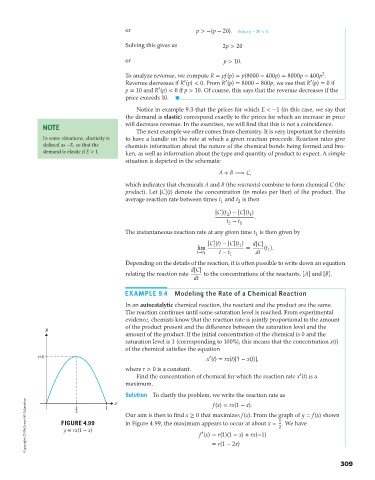
r/4 x (t) = rx(t)[1 − x(t)],
where r > 0 is a constant.
′
Find the concentration of chemical for which the reaction rate x (t)isa
maximum.
Solution To clarify the problem, we write the reaction rate as
Copyright © McGraw-Hill Education FIGURE 4.99 Our aim is then to find x ≥ 0 that maximizes f(x). From the graph of y = f(x) shown
x
f(x) = rx(1 − x).
1
1
2
1
in Figure 4.99, the maximum appears to occur at about x = .Wehave
2
y = rx(1 − x)
′
f (x) = r(1)(1 − x) + rx(−1)
= r(1 − 2x)
309