Page 676 - The Toxicology of Fishes

656 The Toxicology of Fishes

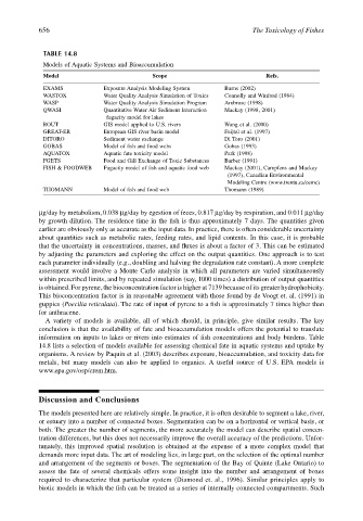
TABLE 14.8
Models of Aquatic Systems and Bioaccumulation
Model Scope Refs.
EXAMS Exposure Analysis Modeling System Burns (2002)
WASTOX Water Quality Analysis Simulation of Toxics Connolly and Winford (1984)
WASP Water Quality Analysis Simulation Program Ambrose (1998)
QWASI Quantitative Water Air Sediment Interaction Mackay (1998, 2001)
fugacity model for lakes
ROUT GIS model applied to U.S. rivers Wang et al. (2000)
GREAT-ER European GIS river basin model Feijtel et al. (1997)
DITORO Sediment water exchange Di Toro (2001)
GOBAS Model of fish and food webs Gobas (1993)
AQUATOX Aquatic fate toxicity model Park (1998)
FGETS Food and Gill Exchange of Toxic Substances Barber (1991)
FISH & FOODWEB Fugacity model of fish and aquatic food web Mackay (2001), Campfens and Mackay
(1997), Canadian Environmental
Modeling Centre (www.trentu.ca/cemc)
THOMANN Model of fish and food web Thomann (1989)

µg/day by metabolism, 0.038 µg/day by egestion of feces, 0.817 µg/day by respiration, and 0.011 µg/day
by growth dilution. The residence time in the fish is thus approximately 7 days. The quantities given
earlier are obviously only as accurate as the input data. In practice, there is often considerable uncertainty
about quantities such as metabolic rates, feeding rates, and lipid contents. In this case, it is probable
that the uncertainty in concentrations, masses, and fluxes is about a factor of 3. This can be estimated
by adjusting the parameters and exploring the effect on the output quantities. One approach is to test
each parameter individually (e.g., doubling and halving the degradation rate constant). A more complete
assessment would involve a Monte Carlo analysis in which all parameters are varied simultaneously
within prescribed limits, and by repeated simulation (say, 1000 times) a distribution of output quantities
is obtained. For pyrene, the bioconcentration factor is higher at 7139 because of its greater hydrophobicity.
This bioconcentration factor is in reasonable agreement with those found by de Voogt et. al. (1991) in
guppies (Poecilia reticulata). The rate of input of pyrene to a fish is approximately 7 times higher than
for anthracene.
A variety of models is available, all of which should, in principle, give similar results. The key
conclusion is that the availability of fate and bioaccumulation models offers the potential to translate
information on inputs to lakes or rivers into estimates of fish concentrations and body burdens. Table
14.8 lists a selection of models available for assessing chemical fate in aquatic systems and uptake by
organisms. A review by Paquin et al. (2003) describes exposure, bioaccumulation, and toxicity data for
metals, but many models can also be applied to organics. A useful source of U.S. EPA models is
www.epa.gov/osp/crem.htm.

Discussion and Conclusions
The models presented here are relatively simple. In practice, it is often desirable to segment a lake, river,
or estuary into a number of connected boxes. Segmentation can be on a horizontal or vertical basis, or
both. The greater the number of segments, the more accurately the model can describe spatial concen-
tration differences, but this does not necessarily improve the overall accuracy of the predictions. Unfor-
tunately, this improved spatial resolution is obtained at the expense of a more complex model that
demands more input data. The art of modeling lies, in large part, on the selection of the optimal number
and arrangement of the segments or boxes. The segmentation of the Bay of Quinte (Lake Ontario) to
assess the fate of several chemicals offers some insight into the number and arrangement of boxes
required to characterize that particular system (Diamond et. al., 1996). Similar principles apply to
biotic models in which the fish can be treated as a series of internally connected compartments. Such