Page 671 - The Toxicology of Fishes

Exposure Assessment and Modeling in the Aquatic Environment 651

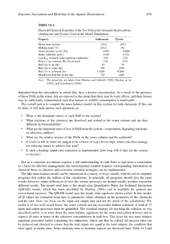
TABLE 14.3
Physical/Chemical Properties of the Two Polycyclic Aromatic Hydrocarbons
(Anthracene and Pyrene) Used in the Model Simulations
Property Anthracene Pyrene
Molar mass (g/mol) 178.2 202.3
Melting point (°C) 216.2 156
Vapor pressure (solid) (Pa) 0.001 0.0006
3
Water solubility (g/m ) 0.045 0.132
Log K OW (octanol–water partition coefficient) 4.54 5.18
3
Henry’s law constant (H) (Pa m /mol) 3.96 0.92
Half-life in air (hr) 55 55
Half-life in water (hr) 550 1700
Half-life in sediment (hr) 17,000 55,000
Metabolism half-life in fish (hr) 720 1080
Note: The properties are taken from Mackay and Callcott (1998), Mackay et. al.
(1992), and Verschueren (1996).

deposited from the atmosphere in which they have a known concentration. As a result of the presence
of these PAHs in the water, fish are exposed to the extent that there may be toxic effects, and their tissues
may be sufficiently contaminated such that human or wildlife consumption is inadvisable.
The overall task is to compile the mass balance model for this system for both chemicals. If this can
be done, it will help answer such questions as:

• What is the dominant source of each PAH to the system?
• What fractions of the chemical are dissolved and sorbed in the water column and are thus
different in bioavailability?
• What are the important rates of loss of PAH from the system—evaporation, degrading reactions,
or advective outflow?
• What are the relative masses of the PAHs in the water column and the sediment?
• If levels in fish or water are judged to be a factor of (say) 10 too high, what is the best strategy
for reducing inputs to achieve this goal?
• If such a loading (input rate) reduction is implemented, how long will it take for the system
to recover?

Just as a corporate accountant requires a full understanding of cash flows to and from a corporation
as a basis for effective management, the environmental scientist requires corresponding information on
chemical flows so effective and economic remedial strategies can be implemented.
The lake mass balance model can be constructed in a variety of ways, usually with the aid of computer
programs that reduce the tedium of the calculations. In principle, all programs should give the same
results; however, minor differences in how the various processes are treated usually produce somewhat
different results. The model used here is the steady-state Quantitative Water Air Sediment Interaction
(QWASI) model, which has been described by Mackay (2001) and is available for general use
(www.trentu.ca/cemc). The QWASI model uses the steady-state equations shown earlier. In this model,
all D values are estimated from data or parameter values obtained on the properties of the chemicals
and the lake. Here, we focus on the input and output data and not the detail of the calculations. The
model is of two well-mixed boxes: the water column and the accessible bottom sediment. A total of 17
input and output processes must be quantified. The essential strategy for reaching the solution, as was
described earlier, is to write down the mass balance equations for the water and sediment boxes and to
express all rates in terms of the unknown concentrations in each box. This gives the two mass balance
equations presented earlier containing two unknowns, which can thus be solved. All process rates can
be deduced and checked to ensure that the total inputs are equal to the total outputs, the condition that
must apply at steady state. Some unsteady-state or dynamic aspects are discussed later. Table 14.2 and