Page 670 - The Toxicology of Fishes

650 The Toxicology of Fishes

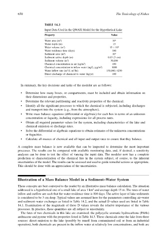
TABLE 14.2
Input Data Used in the QWASI Model for the Hypothetical Lake
Property Value
2
Water area (m ) 10 6
Water depth (m) 15
3
Water volume (m ) 15 × 10 6
Water residence time (days) 100
2
Sediment area (m ) 10 6
Sediment active depth (m) 0.03 (3 cm)
3
Sediment volume (m ) 30,000
3
Chemical concentration in air (ng/m ) 100
3
Chemical concentration in inflow water (ng/L; µg/m ) 1000
3
3
Water inflow rate (m /d; m /hr) 150,000; 6250
Direct discharge of chemical to water (kg/yr) 100
In summary, the key decisions and tasks of the modeler are as follows:
• Determine how many boxes, or compartments, must be included and obtain information on
their dimensions and properties.
• Determine the relevant partitioning and reactivity properties of the chemical.
• Identify all the significant processes to which the chemical is subjected, including discharges
and transport into the system (e.g., from the atmosphere).
• Write mass balance equations (differential or algebraic) for each box in terms of an unknown
concentration or fugacity, including expressions for all process rates.
• Obtain all required parameter values for the system, including characteristics of the lake and
chemical emission or discharge rates.
• Solve the differential or algebraic equations to obtain estimates of the unknown concentrations
or fugacities.
• Calculate all masses of chemical and all input and output rates to ensure that they balance.

A complete mass balance is now available that can be inspected to determine the most important
processes. The results can be compared with available monitoring data, and, if desired, a sensitivity
analyses can be done to test the effect of varying the input data. The modeler now has a complete
prediction or characterization of the chemical fate in the system subject, of course, to the inherent
uncertainties of the model. The results can be assessed and used to guide remedial actions as appropriate.
This should be done with an appreciation of the uncertainties.

Illustration of a Mass Balance Model in a Sediment–Water System

These concepts are best conveyed to the reader by an illustrative mass balance calculation. The situation
addressed is a hypothetical one of a small lake of area 1 km and average depth 15 m. The rates of water
2
inflow and outflow are such that the water residence time is 100 days. The active layer of lake sediments
is considered to be 3 cm deep. Typical values are assumed here for the parameters controlling air–water
and sediment–water exchanges as listed in Table 14.2, and the actual D values used are listed in Table
14.1. Examination of the magnitude of these D values reveals the relative importance of the various
processes. In practice, these quantities are all subject to uncertainty.
The fates of two chemicals in this lake are examined: the polycyclic aromatic hydrocarbons (PAHs)
anthracene and pyrene with the properties listed in Table 14.3. These chemicals enter the lake from three
sources: direct emission to the lake (possibly by runoff from contaminated soil or from an industrial
operation), both chemicals are present in the inflow water at relatively low concentrations, and both are