Page 342 - Linear Models for the Prediction of Animal Breeding Values 3rd Edition

j/2 r
−12
1 () ( j − 2 r)! j−2 r
Pt() = j ∑ t
j
2 r=0 rj !( − r)!( − 2 r)!
j
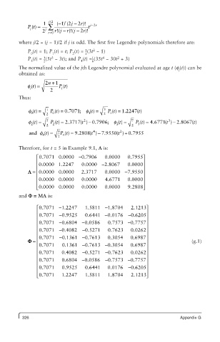
where j/2 = (j − 1)/2 if j is odd. The first five Legendre polynomials therefore are:
2
P (t) = 1; P (t) = t; P (t) = (3t − 1)
1
0 1 2 2
4
3
2
P (t) = (5t − 3t); and P (t) = (35t − 30t + 3)
1
1
3 2 4 8
The normalized value of the jth Legendre polynomial evaluated at age t (f (t)) can be
j
obtained as:
f t() = 2 n + 1 Pt()
j j
2
Thus:
f () = 1 P () = 0 7071; f () = 3 P () = 1 2247( )
.
t
t
t
.
t
t
0 2 0 1 2 1
f () = 5 P () = 2 3717. ( ) - 0 7906; ( ) = 7 P ( ) = 4 6771( ) - 2 8067( )
2
3
t
.
.
t
t
t
.
t
t
2
t
2 2 2 f 3 2 3
2
4
t
t
t
and f (()t = 9 P () = 9 .2808 ( ) - 7 .9550 ( ) + 0 .7955
4 2 4
Therefore, for t = 5 in Example 9.1, L is:
⎡ 0.7071 0.0000 −0.7906 0.0000 0.7955⎤
⎢ ⎥
⎢ 0.0000 1.2247 0.0000 −2.80667 0.0000 ⎥
⎢
L = 0.0000 0.0000 2.3717 0.0000 − 7.9550⎥
⎢ ⎥
⎢ 0.0000 0.0000 0.0000 4 4.6771 0.0000 ⎥
⎢ ⎣ 0.0000 0.0000 0.0000 0.0000 9.2808 ⎥ ⎥ ⎦
and F = ML is:
⎡ 0 7071 −1 2247 1 5811 −1 8704 2 1213⎤
.
.
.
.
.
⎢ − ⎥
.
.
.
.
⎢ 0 7071 −0 9525 0 6441 −0.00176 0 6205 ⎥ ⎥
⎢ 0 7071 − 0 6804 − 0 0586 0 7573 − 0 7757⎥
.
.
.
.
.
⎢ ⎥
.
.
.
⎢ 0 7071 − 0 4082 − −0 5271 0 7623 0 0262 ⎥
.
.
⎢ 0 7071 −0 1361 −0 7613 0 3054 0 6987 ⎥
.
.
.
.
.
F = ⎢ ⎥ (g.1)
.
.
.
⎢ 0 7071 0 0 1361 − 0 7613 − 0 3054 0 6987 ⎥
.
.
⎢ 0 7071 0 4082 − 0 5271 − 0 7623 0 0262 ⎥
2
.
.
.
.
.
⎢ ⎥
⎢ 0 7071 0 6804 − 0 0586 − 0 7573 − 0 7757⎥
.
.
.
.
.
⎢ ⎥
.
.
.
.
.
6
⎢ 0 7071 0 9525 0 6441 0 0176 − 0 6205 ⎥
⎢ ⎣ 0 7071 1 2247 1 5811 1 8704 2 1213⎥ ⎦
.
.
.
.
.
326 Appendix G