Page 337 - Linear Models for the Prediction of Animal Breeding Values 3rd Edition

−1
Partitioning Q and Q as specified above gives the following matrices:
⎡ 0.1659⎤ ⎡− 0.0792⎤
Q = ⎢ ⎥ , Q = ⎢ ⎥ ,
v m
⎣ 0.0168 ⎦ ⎣ 0.1755 ⎦
[
v
Q = 5.76651 2.6006] and Q m = [− 0.5503 5.4495]
From the residual covariance matrix in Section E.1:
−1
R R = 11/40 = 0.275
mv vv
The matrices Q and Q , respectively, are:
1 2
.
é0 1659. ù - é 0 0792. ù é 0 1441ù
Q = + 0 275 =
.
1 ê ú ê ú ê ú
ë 0 0168 û ë 0 1755 û ë 0 06544 û
.
.
.
and:
− ⎡ ⎡ 0.0792⎤ − ⎡ 0.0792⎤ ⎤
Q = ⎢ ⎢ ⎥ − [ 0.5503 5.4495] − ⎢ ⎥ 0.275 [5.7651 2.6006 ]⎥
2
⎣ ⎣ 0.1755 ⎦ ⎣ ⎣ 0.1755 ⎦ ⎦
⎡ 0.1691 − 0.3750⎤
= ⎢ ⎥
⎣ − 0.3748 0 0.8309 ⎦
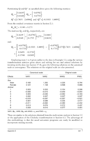
Employing steps 1 to 4 given earlier to the data in Example 5.2, using the various
transformation matrices given above and solving for sex and animal solutions by
iterating on the data (see Section 17.4), gave the following solutions on the canonical
scale at convergence. The solutions on the original scale are also presented.

Canonical scale Original scale
Effects VAR1 VAR2 WWG PWG

Sex
Male 0.180 1.265 4.326 6.794
Female 0.124 1.108 3.598 5.968
Animal
1 0.003 0.053 0.154 0.288
2 −0.006 −0.010 −0.059 −0.054
3 0.003 −0.030 −0.062 −0.163
4 0.002 0.007 0.027 0.037
5 −0.010 −0.097 −0.307 −0.521
6 0.001 0.088 0.235 0.477
7 −0.011 −0.084 −0.280 −0.452
8 0.013 0.076 0.272 0.407
9 0.009 0.010 0.077 0.051
VAR1, Qy , VAR2, Qy with WWG = y and PWG = y .
1 2 1 2
These are similar to the solutions obtained from the multivariate analysis in Section 5.3
or the application of the Cholesky transformation in Section 6.3. The advantage of
this methodology is that the usual univariate programs can easily be modified to
incorporate missing records.

Appendix E 321