Page 338 - Linear Models for the Prediction of Animal Breeding Values 3rd Edition

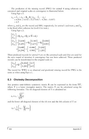
The prediction of the missing record (PWG) for animal 4 using solutions on
canonical and original scales at convergence is illustrated below.
Using Eqn e.1:
ˆ
ˆ
−1
y = b + aˆ + R R (y − b − aˆ )
42 12 42 mv vv 41 11 41
= 6.836 + 0.016 + 0.275(4.5 − 4.366 − 0.007)
= 6.9
ˆ
where y and aˆ are the record and EBV, respectively, for animal i and trait j, and b
ij ij kj
is the fixed effect solution for level k for trait j.
Using Eqn e.2:
ˆ y ⎡ * 41 ⎤
a
⎢ ⎥ = Q 1 y + Q 2 (x b′ ˆ * + )
ˆ *
4
41
⎣ ˆ y * 42 ⎦
ˆ y ⎡ * 41 ⎤ ⎡0.648 ⎤ ⎡0.183 ⎤ ⎡0.000⎤
⎢ ⎥ ⎥ = ⎢ ⎥ + Q 2 ⎢ ⎥ + Q 2 ⎢ ⎥
⎣ ˆ y * 42 ⎦ ⎣ 0.294 ⎦ ⎣ 1.273 ⎦ ⎣ ⎣ 0.003 ⎦
⎡0.648 ⎤ ⎡ 0.446− ⎤ ⎡ 0.202⎤
= ⎢ ⎥ + ⎢ ⎥ = ⎢ ⎥
⎣ 0.294 ⎦ ⎣ 0.989 ⎦ ⎣ 1.2883 ⎦
These predicted records for animal 4 are on the canonical scale and they are used for
the next round of iteration if convergence has not been achieved. These predicted
records can be transformed to the original scale as:
ˆ y ⎡ 41 ⎤ −1 ⎡0.202 ⎤ ⎡4.5 ⎤
=
⎢ ⎥ = Q ⎢ ⎥ ⎢ ⎥
⎣ ˆ y 42⎦ ⎣ 1.283 ⎦ ⎣ 6.9 ⎦
The record for WWG is as observed and predicted missing record for PWG is the
same as when using Eqn e.1.

E.3 Cholesky Decomposition

Any positive semi-definite symmetric matrix R can be expressed in the form TT′,
where T is a lower triangular matrix. The matrix T can be calculated using the
following formulae. The ith diagonal element of T is calculated as:

i−1
ii t = r − ij t ∑ 2
ii
j=1
and the lower off-diagonal element of the ith row and the kth column of T as:

⎛ k 1 ⎞
−
1
ik t = r ⎜ ik − t ∑ ij kj t ⎟
t kk ⎝ j=1 ⎠

322 Appendix E