Page 335 - Linear Models for the Prediction of Animal Breeding Values 3rd Edition

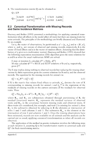
4. The transformation matrix Q can be obtained as:
Q = L′P
é 0.1659 - 0.0792ù é 5.7651 2.6006ù
Q = ê ú and Q - 1 = ê ú
ë 0.0168 0.1755 û ë - -0.5503 5.4495 û

E.2 Canonical Transformation with Missing Records
and Same Incidence Matrices

Ducrocq and Besbes (1993) presented a methodology for applying canonical trans-
formation when all effects in the model affect all traits but there are missing traits for
some animals. The principles of the methodology are briefly discussed and illustrated
by an example.
Let y, the vector of observations, be partitioned as y′ = [y , y ] and u = [b′, a′],
v m
where y and y are vectors of observed and missing records, respectively, b is the
v m
vector of fixed effects and a is the vector of random effects. Assuming that the distri-
bution of y given u is multivariate normal, Ducrocq and Besbes (1993) showed that
the following expectation maximization (EM) algorithm gives the same solutions for
a and b as when the usual multivariate MME are solved:

E step: at iteration k, calculate y = E[y|y , uˆ ]
[k]
[k]
ˆ
v
M step: calculate u ˆ [k+1] = BLUE and BLUP solutions of b and a, respectively,
given y ˆ [k]
The E step implies doing nothing to observed records but replacing the missing obser-
vations by their expectation given the current solutions for b and a, and the observed
records. The equation for the missing records for animal i is:
[k]
[k]
y = x ′ b + aˆ [k] + e ˆ [k] (e.1)
ˆ
im im im im
If X is the matrix that relates fixed effects to animals, x′ denotes the row of X
im
corresponding to missing records for animal i and e ˆ [k] is the regression of the
im
residuals of missing records on the current estimates of the residuals for observed
traits. Thus:
−1
[k]
[k]
[k]
[k]
e = E[e |y , u = uˆ ] = R R [y − x′ b − a ]
ˆ
ˆ
im im iv mv vv iv iv iv
where R and R are submatrices obtained through partitioning of R, the
mv vv
residual covariance matrix. R represents the residual variance of observed
vv
traits and R is the covariance between missing traits and observed traits. If
mv
three traits are considered, for example, and trait 2 is missing for animal i, then
R is the submatrix obtained by selecting in R the elements at intersection of
vv
rows 1 and 3 and columns 1 and 3. The submatrix R is the element at the
mv
intersection of row 2 and columns 1 and 3. Once the missing observations have
been estimated, records are now available on all animals and the analysis can be
carried out as usual, applying canonical transformation as when all records are
observed.
The application of the method in genetic evaluation involves the following steps
at each iteration k, assuming Q is the transformation matrix to canonical scale and
Q the back-transforming matrix:
−1
Appendix E 319